Buffers are solutions that maintain a relatively constant pH when an acid or a base is added. They therefore protect, or “buffer,” other molecules in solution from the effects of the added acid or base. Buffers contain either a weak acid (HA) and its conjugate base (A−) or a weak base (B) and its conjugate acid (BH+), and they are critically important for the proper functioning of biological systems. In fact, every biological fluid is buffered to maintain its physiological pH.

The Common Ion Effect with Acids and Bases

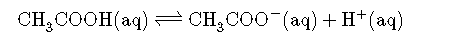
To understand how buffers work, let’s look first at how the ionization equilibrium of a weak acid is affected by adding either the conjugate base of the acid or a strong acid (a source of H+). Le Chatelier’s principle can be used to predict the effect on the equilibrium position of the solution. A typical buffer used in biochemistry laboratories contains acetic acid and a salt such as sodium acetate. The dissociation reaction of acetic acid is as follows:

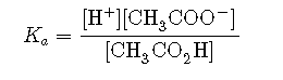
and the equilibrium constant expression is as follows:

Sodium acetate (CH3CO2Na) is a strong electrolyte that ionizes completely in aqueous solution to produce Na+ and CH3CO−2 ions. If sodium acetate is added to a solution of acetic acid, Le Chatelier’s principle predicts that the equilibrium will shift to the left, consuming some of the added CH3COO− and some of the H+ ions originally present in solution.

Because Na+ is a spectator ion, it has no effect on the position of the equilibrium and can be ignored. The addition of sodium acetate produces a new equilibrium composition, in which [H+] is less than the initial value. Because [H+] has decreased, the pH will be higher. Thus adding a salt of the conjugate base to a solution of a weak acid increases the pH. This makes sense because sodium acetate is a base, and adding any base to a solution of a weak acid should increase the pH.

If we instead add a strong acid such as HCl to the system, [H+] increases. Once again the equilibrium is temporarily disturbed, but the excess H+ ions react with the conjugate base (CH3CO−2), whether from the parent acid or sodium acetate, to drive the equilibrium to the left. The net result is a new equilibrium composition that has a lower [CH3CO−2] than before. In both cases, only the equilibrium composition has changed; the ionization constant Ka for acetic acid remains the same. Adding a strong electrolyte that contains one ion in common with a reaction system that is at equilibrium, in this case CH3CO−2, will therefore shift the equilibrium in the direction that reduces the concentration of the common ion. The shift in equilibrium is via the common ion effect.

Adding a common ion to a system at equilibrium affects the equilibrium composition, but not the ionization constant.

Now let’s suppose we have a buffer solution that contains equimolar concentrations of a weak base (B) and its conjugate acid (BH+). The general equation for the ionization of a weak base is as follows:

If the equilibrium constant for the reaction as written is small, for example Kb=10−5, then the equilibrium constant for the reverse reaction is very large: K=1Kb=105. Adding a strong base such as OH− to the solution therefore causes the equilibrium to shift to the left, consuming the added OH−. As a result, the OH− ion concentration in solution remains relatively constant, and the pH of the solution changes very little. Le Chatelier’s principle predicts the same outcome: when the system is stressed by an increase in the OH− ion concentration, the reaction will proceed to the left to counteract the stress.

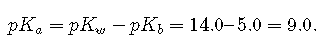
If the pKb of the base is 5.0, the pKa of its conjugate acid is

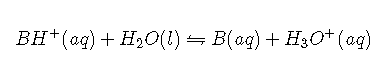
Thus the equilibrium constant for ionization of the conjugate acid is even smaller than that for ionization of the base. The ionization reaction for the conjugate acid of a weak base is written as follows:

Again, the equilibrium constant for the reverse of this reaction is very large: K = 1/Ka = 109. If a strong acid is added, it is neutralized by reaction with the base as the reaction  shifts to the left. As a result, the H+ ion concentration does not increase very much, and the pH changes only slightly. In effect, a buffer solution behaves somewhat like a sponge that can absorb H+ and OH− ions, thereby preventing large changes in pH when appreciable amounts of strong acid or base are added to a solution.

Buffers are characterized by the pH range over which they can maintain a more or less constant pH and by their buffer capacity, the amount of strong acid or base that can be absorbed before the pH changes significantly. Although the useful pH range of a buffer depends strongly on the chemical properties of the weak acid and weak base used to prepare the buffer (i.e., on K), its buffer capacity depends solely on the concentrations of the species in the buffered solution. The more concentrated the buffer solution, the greater its buffer capacity. As illustrated in Figure $1$, when NaOH is added to solutions that contain different concentrations of an acetic acid/sodium acetate buffer, the observed change in the pH of the buffer is inversely proportional to the concentration of the buffer. If the buffer capacity is 10 times larger, then the buffer solution can absorb 10 times more strong acid or base before undergoing a significant change in pH.

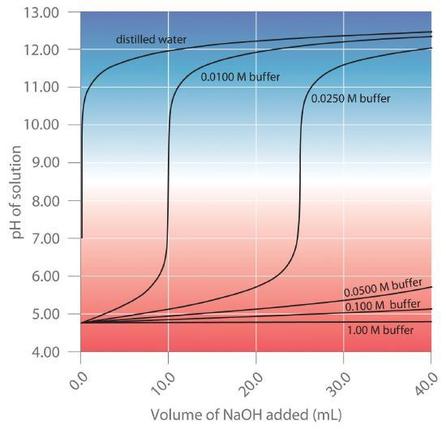
A buffer maintains a relatively constant pH when acid or base is added to a solution. The addition of even tiny volumes of 0.10 M NaOH to 100.0 mL of distilled water results in a very large change in pH. As the concentration of a 50:50 mixture of sodium acetate/acetic acid buffer in the solution is increased from 0.010 M to 1.00 M, the change in the pH produced by the addition of the same volume of NaOH solution decreases steadily. For buffer concentrations of at least 0.500 M, the addition of even 25 mL of the NaOH solution results in only a relatively small change in pH.

Calculating the pH of a Buffer

The pH of a buffer can be calculated from the concentrations of the weak acid and the weak base used to prepare it, the concentration of the conjugate base and conjugate acid, and the pKa or pKb of the weak acid or weak base. 

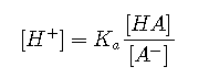
An alternative method frequently used to calculate the pH of a buffer solution is based on a rearrangement of the equilibrium equation for the dissociation of a weak acid. The simplified ionization reaction is HA⇋H++A−, for which the equilibrium constant expression is as follows:

This equation can be rearranged as follows:

Taking the logarithm of both sides and multiplying both sides by −1,

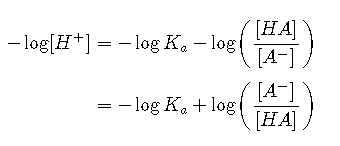
Replacing the negative logarithms

or, more generally,

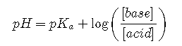
They are both forms of the Henderson-Hasselbalch approximation, named after the two early 20th-century chemists who first noticed that this rearranged version of the equilibrium constant expression provides an easy way to calculate the pH of a buffer solution. In general, the validity of the Henderson-Hasselbalch approximation may be limited to solutions whose concentrations are at least 100 times greater than their Ka values.

There are three special cases where the Henderson-Hasselbalch approximation is easily interpreted without the need for calculations:

• $[base]=[acid]$: Under these conditions,

  

  Because log 1=0,

  

  regardless of the actual concentrations of the acid and base. Recall that this corresponds to the midpoint in the titration of a weak acid or a weak base.

  
  

• $[base]/[acid]=10$, Because log 10=1,

$$

• $[base]/[acid]=100$, Because log 100=2,

Each time we increase the [base]/[acid] ratio by 10, the pH of the solution increases by 1 pH unit. Conversely, if the [base]/[acid] ratio is 0.1, then pH = pKa− 1. Each additional factor-of-10 decrease in the [base]/[acid] ratio causes the pH to decrease by 1 pH unit.

If [base] = [acid] for a buffer, then pH = pKa. Changing this ratio by a factor of 10 either way changes the pH by ±1 unit.

Suppose we had added the same amount of HCl or NaOH solution to 100 mL of an unbuffered solution at pH 3.95 (corresponding to 1.1×10−4 M HCl). In this case, adding 5.00 mL of 1.00 M HCl would lower the final pH to 1.32 instead of 3.70, whereas adding 5.00 mL of 1.00 M NaOH would raise the final pH to 12.68 rather than 4.24. (Try verifying these values by doing the calculations yourself.) Thus the presence of a buffer significantly increases the ability of a solution to maintain an almost constant pH.

The most effective buffers contain equal concentrations of an acid and its conjugate base.

A buffer that contains approximately equal amounts of a weak acid and its conjugate base in solution is equally effective at neutralizing either added base or added acid. This is shown in Figure $2$ for an acetic acid/sodium acetate buffer. Adding a given amount of strong acid shifts the system along the horizontal axis to the left, whereas adding the same amount of strong base shifts the system the same distance to the right. In either case, the change in the ratio of CH3CO−2 to CH3CO2H from 1:1 reduces the buffer capacity of the solution.

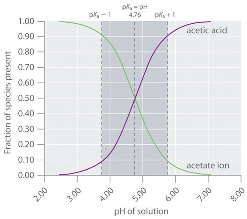
The Relationship between Titrations and Buffers

There is a strong correlation between the effectiveness of a buffer solution and the titration curves discussed in Section 16.5. Consider the schematic titration curve of a weak acid with a strong base shown in Figure $3$. As indicated by the labels, the region around pKa corresponds to the midpoint of the titration, when approximately half the weak acid has been neutralized. This portion of the titration curve corresponds to a buffer: it exhibits the smallest change in pH per increment of added strong base, as shown by the nearly horizontal nature of the curve in this region. The nearly flat portion of the curve extends only from approximately a pH value of 1 unit less than the pKa to approximately a pH value of 1 unit greater than the pKa, which is why buffer solutions usually have a pH that is within ±1 pH units of the pKa of the acid component of the buffer.

This schematic plot of pH for the titration of a weak acid with a strong base shows the nearly flat region of the titration curve around the midpoint, which corresponds to the formation of a buffer. At the lower left, the pH of the solution is determined by the equilibrium for dissociation of the weak acid; at the upper right, the pH is determined by the equilibrium for reaction of the conjugate base with water.

In the region of the titration curve at the lower left, before the midpoint, the acid–base properties of the solution are dominated by the equilibrium for dissociation of the weak acid, corresponding to Ka. In the region of the titration curve at the upper right, after the midpoint, the acid–base properties of the solution are dominated by the equilibrium for reaction of the conjugate base of the weak acid with water, corresponding to Kb. However, we can calculate either Ka or Kb from the other because they are related by Kw.

Blood: A Most Important Buffer

Metabolic processes produce large amounts of acids and bases, yet organisms are able to maintain an almost constant internal pH because their fluids contain buffers. This is not to say that the pH is uniform throughout all cells and tissues of a mammal. The internal pH of a red blood cell is about 7.2, but the pH of most other kinds of cells is lower, around 7.0. Even within a single cell, different compartments can have very different pH values. For example, one intracellular compartment in white blood cells has a pH of around 5.0.

Because no single buffer system can effectively maintain a constant pH value over the entire physiological range of approximately pH 5.0 to 7.4, biochemical systems use a set of buffers with overlapping ranges. The most important of these is the CO2/HCO−3 system, which dominates the buffering action of blood plasma.

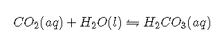
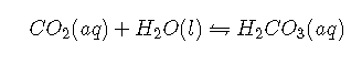
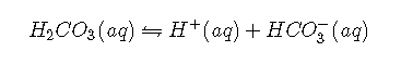
The acid–base equilibrium in the CO2/HCO−3 buffer system is usually written as follows:

with Ka=4.5×10−7 and pKa=6.35  at 25°C. In fact, it is a grossly oversimplified version of the CO2/HCO−3 system because a solution of CO2 in water contains only rather small amounts of H2CO3. Thus it does not allow us to understand how blood is actually buffered, particularly at a physiological temperature of 37°C. As shown, CO2 is in equilibrium with H2CO3, but the equilibrium lies far to the left, with an H2CO3/CO2 ratio less than 0.01 under most conditions:

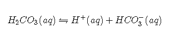
with K'=4.0×10−3 at 37°C. The true pKa of carbonic acid at 37°C is therefore 3.70, not 6.35, corresponding to a Ka of 2.0×10−4, which makes it a much stronger acid than suggests. Adding Equations and canceling H2CO3 from both sides give the following overall equation for the reaction of CO2 with water to give a proton and the bicarbonate ion:

with K′=4.0×10−3(37°C)

with Ka=2.0×10−4(37°C)

with K=8.0×10−7(37°C)

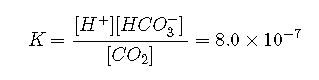
The K value for the reaction  is the product of the true ionization constant for carbonic acid (Ka) and the equilibrium constant (K) for the reaction of CO2(aq) with water to give carbonic acid. The equilibrium equation for the reaction of CO2 with water to give bicarbonate and a proton is therefore

unusual. According to Henry’s law,

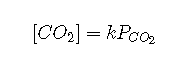
where k is the Henry’s law constant for CO2, which is 3.0×10−5M/mmHg  at 37°C. Substituting this expression for [CO2],

where PCO2 is in mmHg. Taking the negative logarithm of both sides and rearranging,

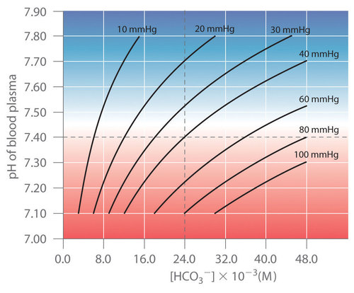
Thus the pH of the solution depends on both the CO2 pressure over the solution and [HCO−3]. Figure $4$ plots the relationship between pH and [HCO−3]under physiological conditions for several different values of PCO2, with normal pH and [HCO−3] values indicated by the dashed lines.

According to Equation, adding a strong acid to the CO2/HCO−3 system causes [HCO−3] to decrease as HCO−3 is converted to CO2. Excess CO2 is released in the lungs and exhaled into the atmosphere, however, so there is essentially no change in PCO2. Because the change in [HCO−3]/PCO2 is small, Equation predicts that the change in pH will also be rather small. Conversely, if a strong base is added, the OH− reacts with CO2 to form [HCO−3], but CO2 is replenished by the body, again limiting the change in both [HCO−3]/PCO2 and pH. The CO2/HCO−3 buffer system is an example of an open system, in which the total concentration of the components of the buffer change to keep the pH at a nearly constant value.

If a passenger steps out of an airplane in Denver, Colorado, for example, the lower PCO2 at higher elevations (typically 31 mmHg at an elevation of 2000 m versus 40 mmHg at sea level) causes a shift to a new pH and [HCO−3]. The increase in pH and decrease in [HCO−3] in response to the decrease in PCO2 are responsible for the general malaise that many people experience at high altitudes. If their blood pH does not adjust rapidly, the condition can develop into the life-threatening phenomenon known as altitude sickness.

Summary

Buffers are solutions that resist a change in pH after adding an acid or a base. Buffers contain a weak acid (HA) and its conjugate weak base (A−). Adding a strong electrolyte that contains one ion in common with a reaction system that is at equilibrium shifts the equilibrium in such a way as to reduce the concentration of the common ion. The shift in equilibrium is called the common ion effect. Buffers are characterized by their pH range and buffer capacity. The useful pH range of a buffer depends strongly on the chemical properties of the conjugate weak acid–base pair used to prepare the buffer (the Ka or Kb), whereas its buffer capacity depends solely on the concentrations of the species in the solution. The pH of a buffer can be calculated using the Henderson-Hasselbalch approximation, which is valid for solutions whose concentrations are at least 100 times greater than their Ka values. Because no single buffer system can effectively maintain a constant pH value over the physiological range of approximately 5 to 7.4, biochemical systems use a set of buffers with overlapping ranges. The most important of these is the CO2/HCO−3 system, which dominates the buffering action of blood plasma.