The methods for dealing with acid-base equilibria that we developed in the earlier units of this series are widely used in ordinary practice. Although many of these involve approximations of various kinds, the results are usually good enough for most purposes. Sometimes, however — for example, in problems involving very dilute solutions, the approximations break down, often because they ignore the small quantities of H+ and OH– ions always present in pure water. In this unit, we look at exact, or "comprehensive" treatment of some of the more common kinds of acid-base equilibria problems.

Strong acid-base systems

The usual definition of a “strong” acid or base is one that is completely dissociated in aqueous solution. Hydrochloric acid is a common example of a strong acid. When HCl gas is dissolved in water, the resulting solution contains the ions H3O+, OH–, and Cl–, but except in very concentrated solutions, the concentration of HCl is negligible; for all practical purposes, molecules of “hydrochloric acid”, HCl, do not exist in dilute aqueous solutions. To specify the concentrations of the three species present in an aqueous solution of HCl, we need three independent relations between them.

LIMITING CONDITIONS

These relations are obtained by observing that certain conditions must always hold for aqueous solutions:

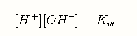
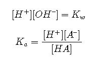
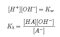
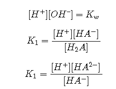
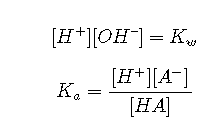
1. The dissociation equilibrium of water must always be satisfied:

   
   

   

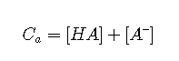
2. The undissociated acid and its conjugate base must be in mass balance. The actual concentrations of the acid and its conjugate base can depend on a number of factors, but their sum must be constant, and equal to the “nominal concentration”, which we designate here as Ca. For a solution of HCl, this equation would be

   
   

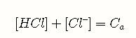
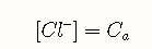
   Because a strong acid is by definition completely dissociated, we can neglect the first term and write the mass balance condition as

   
   

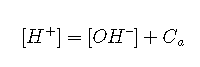
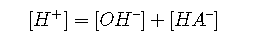
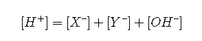
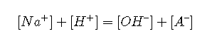
3. In any ionic solution, the sum of the positive and negative electric charges must be zero; in other words, all solutions are electrically neutral. This is known as the electroneutrality principle.

   
   

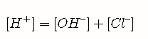
   expression that relates the hydronium ion concentration to 

Ca. This is best done by starting with an equation that relates several quantities and substituting the terms that we want to eliminate. Thus we can get rid of the [Cl–] term by substituting :

The [OH–] term can be eliminated 

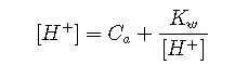
This equation tells us that the hydronium ion concentration will be the same as the nominal concentration of a strong acid as long as the solution is not very dilute. As the acid concentration falls below about 10–6 M, however, the second term predominates; [H+] approaches Kw−−−√ or 10–7M at 25 °C. The hydronium ion concentration can of course never fall below this value; no amount of dilution can make the solution alkaline!

No amount of dilution can make the solution of a strong acid alkaline!

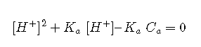
Notice that the Equation is a quadratic equation; in regular polynomial form it would be rewritten as

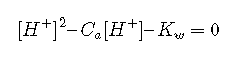
Most practical problems involving strong acids are concerned with more concentrated solutions in which the second term can be dropped, yielding the simple relation

ACTIVITIES AND CONCENTRATED SOLUTIONS OF STRONG ACIDS

In more concentrated solutions, interactions between ions cause their “effective” concentrations, known as their activities, to deviate from their “analytical” concentrations. Thus in a solution prepared by adding 0.5 mole of the very strong acid HClO4 to sufficient water to make the volume 1 liter, freezing-point depression measurements indicate that the concentrations of hydronium and perchlorate ions are only about 0.4 M. This does not mean that the acid is only 80% dissociated; there is no evidence of HClO4 molecules in the solution. What has happened is that about 20% of the H3O+ and ClO4– ions have formed ion-pair complexes in which the oppositely-charged species are loosely bound by electrostatic forces. Similarly, in a 0.10 M solution of hydrochloric acid, the activity of H+ is 0.81, or only 81% of its concentration. (See the green box below for more on this.)

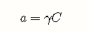
Activities are important because only these work properly in equilibrium calculations. The relation between the concentration of a species and its activity is expressed by the activity coefficient γ:

As a solution becomes more dilute, γ approaches unity. At ionic concentrations below about 0.001 M, concentrations can generally be used in place of activities with negligible error. Recall that pH is defined as the negative logarithm of the hydrogen ion activity, not its concentration.

Activities of single ions cannot be determined, so activity coefficients in ionic solutions are always the average, or mean, of those for all ionic species present. This quantity is denoted as γ±.

At very high concentrations, activities can depart wildly from concentrations. This is a practical consideration when dealing with strong mineral acids which are available at concentrations of 10 M or greater. In a 12 M solution of hydrochloric acid, for example, the mean ionic activity coefficient* is 207. This means that under these conditions with [H+] = 12, the activity {H+} = 2500, corresponding to a pH of about –3.4, instead of –1.1 as might be predicted if concentrations were being used. These very high activity coefficients also explain another phenomenon: why you can detect the odor of HCl over a concentrated hydrochloric acid solution even though this acid is supposedly "100% dissociated".

At these high concentrations, a pair of "dissociated" ions H+ and Cl– will occasionally find themselves so close together that they may momentarily act as an HCl unit; some of these may escape as \(HCl(g)\) before thermal motions break them up again. Under these conditions, “dissociation” begins to lose its meaning so that in effect, dissociation is no longer complete. Although the concentration of \(HCl(aq)\) will always be very small, its own activity coefficient can be as great as 2000, which means that its escaping tendency from the solution is extremely high, so that the presence of even a tiny amount is very noticeable.

Weak monoprotic acids and bases

Most acids are weak; there are hundreds of thousands of them, whereas there are no more than a few dozen strong acids. We can treat weak acid solutions in exactly the same general way as we did for strong acids. The only difference is that we must now include the equilibrium expression for the acid. We will start with the simple case of the pure acid in water, and then go from there to the more general one in which strong cations are present. In this exposition, we will refer to “hydrogen ions” and [H+] for brevity, and will assume that the acid HA dissociates into H+ and its conjugate base A−.

Pure acid in water

In addition to the species H+, OH–, and A− which we had in the strong-acid case, we now have the undissociated acid HA; four variables, requiring four equations.

• Equilibria

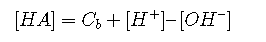
• Mass balance

• Charge balance

To eliminate [HA] , we solve it for this term, and substitute the resulting expression into the numerator:

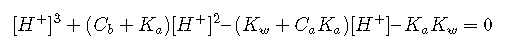
The latter equation is simplified by multiplying out and replacing [H+][OH–] with Kw. We then get rid of the [OH–] term by replacing it with Kw/[H+]

Rearranged into standard polynomial form, this becomes

For most practical applications, we can make approximations that eliminate the need to solve a cubic equation.

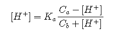
Approximation 1: Neglecting Hydroxide Population

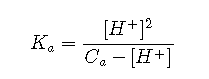
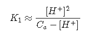
Unless the acid is extremely weak or the solution is very dilute, the concentration of OH– can be neglected in comparison to that of [H+]. If we assume that [OH–] ≪ [H+], then Equation can be simplified to

which is a quadratic equation:

and thus, from the quadratic formula,

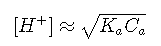
Approximation 2: Very Concentrated Acids

If the acid is fairly concentrated (usually more than 10–3 M), a further simplification can frequently be achieved by making the assumption that [H+]≪Ca. This is justified when most of the acid remains in its protonated form [HA], so that relatively little H+ is produced. In this event,  reduces to

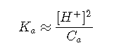
or

Approximation 3: Very Weak and Acidic

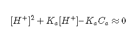
If the acid is very weak or its concentration is very low, the H+ produced by its dissociation may be little greater than that due to the ionization of water. However, if the solution is still acidic, it may still be possible to avoid solving the cubic equation  by assuming that the term ([H+]−[OH–])≪Ca in Equation:

This can be rearranged into standard quadratic form

For dilute solutions of weak acids, an exact treatment may be required. With the aid of a computer or graphic calculator, solving a cubic polynomial is now far less formidable than it used to be. However, round-off errors can cause these computerized cubic solvers to blow up; it is generally safer to use a quadratic approximation.

Weak bases

The weak bases most commonly encountered are:

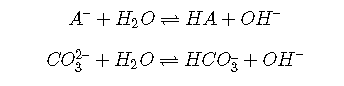
• anions A– of weak acids:

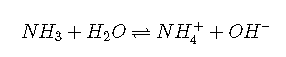
• ammonia

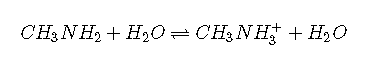
• amines, e.g. methylamine

Solution of an anion of a weak acid

Note that, in order to maintain electroneutrality, anions must be accompanied by sufficient cations to balance their charges. Thus for a Cb M solution of the salt NaA in water, we have the following conditions:

• Species

Na+, A–, HA, H2O, H+, OH–

• Equilibria

• Mass balance

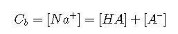
• Charge balance

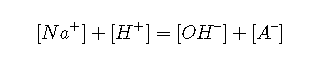
Replacing the [Na+] term in Equation by Cb and combining with Kw and the mass balance, a relation is obtained that is analogous to that for weak acids:

The approximations

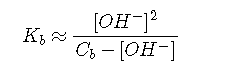
and

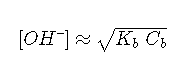
can be derived in a similar manner.

Mixtures of Acids

Many practical problems relating to environmental and physiological chemistry involve solutions containing more than one acid. In this section, we will restrict ourselves to a much simpler case of two acids, with a view toward showing the general method of approaching such problems by starting with charge- and mass-balance equations and making simplifying assumptions when justified. In general, the hydrogen ions produced by the stronger acid will tend to suppress dissociation of the weaker one, and both will tend to suppress the dissociation of water, thus reducing the sources of H+ that must be dealt with.

Consider a mixture of two weak acids HX and HY; their respective nominal concentrations and equilibrium constants are denoted by Cx , Cy , Kx  and Ky ,

Starting with the charge balance expression

We use the equilibrium constants to replace the conjugate base concentrations with expressions of the form

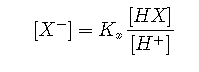
to yield

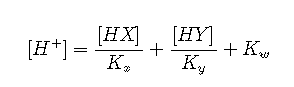
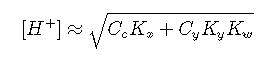
If neither acid is very strong or very dilute, we can replace equilibrium concentrations with nominal concentrations:

Equilibria of Polyprotic Acids

Owing to the large number of species involved, exact solutions of problems involving polyprotic acids can become very complicated. Thus for phosphoric acid H3PO4, the three "dissociation" steps yield three conjugate bases:

Fortunately, it is usually possible to make simplifying assumptions in most practical applications. In the section that follows, we will show how this is done for the less-complicated case of a diprotic acid. A diprotic acid HA can donate its protons in two steps, yielding first a monoprotonated species HA– and then the completely deprotonated form A2–.

Since there are five unknowns (the concentrations of the acid, of the two conjugate bases and of H+ and OH–), we need five equations to define the relations between these quantities. These are

• Equilibria

• Mass balance

• Charge balance

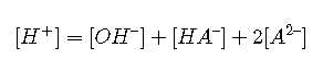
(It takes 2 moles of H+ to balance the charge of 1 mole of A2–)

Solving these five equations simultaneously for K1 yields the rather intimidating expression

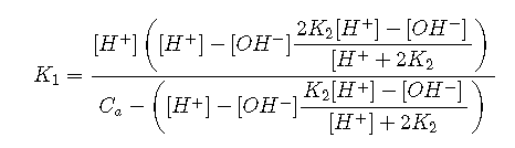
which is of little practical use except insofar as it provides the starting point for various simplifying approximations.

If the solution is even slightly acidic, then ([H+] – [OH–]) ≈ [H+] and

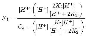
For any of the common diprotic acids, K2 is much smaller than K1. If the solution is sufficiently acidic that K2≪[H+], then a further simplification can be made that removes K2 from Equation ; this is the starting point for most practical calculations.

Finally, if the solution is sufficiently concentrated and K1 sufficiently small so that [H+]≪Ca, then Equationreduces to:

Acid with conjugate base: Buffer solutions

Solutions containing a weak acid together with a salt of the acid are collectively known as buffers. When they are employed to control the pH of a solution (such as in a microbial growth medium), a sodium or potassium salt is commonly used and the concentrations are usually high enough for the Henderson-Hasselbalch equation to yield adequate results.

Exact solution

In this section, we will develop an exact analytical treatment of weak acid-salt solutions, and show how the H–H equation arises as an approximation. A typical buffer system is formed by adding a quantity of strong base such as sodium hydroxide to a solution of a weak acid HA. Alternatively, the same system can be made by combining appropriate amounts of a weak acid and its salt NaA. A system of this kind can be treated in much the same way as a weak acid, but now with the parameter Cb in addition to Ca.

• Species

Na+, A–, HA, H2O, H+, OH–

• Equilibria

• Mass balance

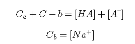
• Charge balance

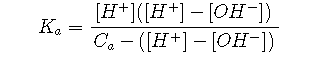
Substituting equations and yields an expression for [A–]:

Inserting this into Equation and solving for [HA] yields

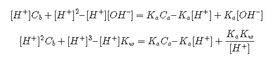
Finally, we substitute these last two expressions into the equilibrium constant :

which becomes cubic in [H+] when [OH–] is replaced by (Kw / [H+]).

Approximations

In almost all practical cases it is possible to make simplifying assumptions. Thus if the solution is known to be acidic or alkaline, then the [OH–] or [H+] terms can be neglected. In acidic solutions, for example, Equation becomes

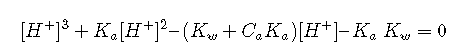
which can be rearranged into a quadratic in standard polynomial form:

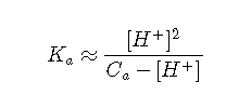
If the concentrations Ca and Cb are sufficiently large, it may be possible to neglect the [H+] terms entirely, leading to the commonly-seen Henderson-Hasselbalch Approximation.

It's important to bear in mind that the Henderson-Hasselbalch Approximation is an "approximation of an approximation" that is generally valid only for combinations of Ka and concentrations that fall within the colored portion of this plot.

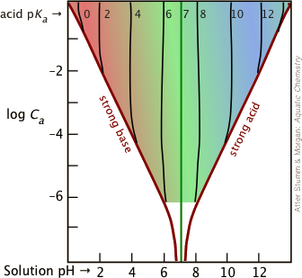
Most buffer solutions tend to be fairly concentrated, with Ca and Cb typically around 0.01 - 0.1 M. For more dilute buffers and larger Ka's that bring you near the boundary of the colored area, it is safer to start with the last Equation.