The rate laws we have seen thus far relate the rate and the concentrations of reactants. We can also determine a second form of each rate law that relates the concentrations of reactants and time. These are called integrated rate laws. We can use an integrated rate law to determine the amount of reactant or product present after a period of time or to estimate the time required for a reaction to proceed to a certain extent. For example, an integrated rate law is used to determine the length of time a radioactive material must be stored for its radioactivity to decay to a safe level.

Using calculus, the differential rate law for a chemical reaction can be integrated with respect to time to give an equation that relates the amount of reactant or product present in a reaction mixture to the elapsed time of the reaction. This process can either be very straightforward or very complex, depending on the complexity of the differential rate law. For purposes of discussion, we will focus on the resulting integrated rate laws for first-, second-, and zero-order reactions.

First-Order Reactions

An equation relating the rate constant k$k$ to the initial concentration [A]0 and the concentration [A]t$[A{]}_t$ present after any given time t$t$ can be derived for a first-order reaction and shown to be:

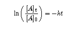
or alternatively

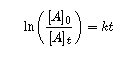
or

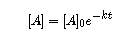
We can use integrated rate laws with experimental data that consist of time and concentration information to determine the order and rate constant of a reaction. The integrated rate law can be rearranged to a standard linear equation format:

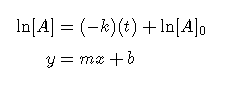
A plot of ln[A] versus t$t$ for a first-order reaction is a straight line with a slope of −k and an intercept of ln[A]0. If a set of rate data are plotted in this fashion but do not result in a straight line, the reaction is not first order in A.

Second-Order Reactions

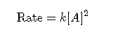
The equations that relate the concentrations of reactants and the rate constant of second-order reactions are fairly complicated. We will limit ourselves to the simplest second-order reactions, namely, those with rates that are dependent upon just one reactant’s concentration and described by the differential rate law:

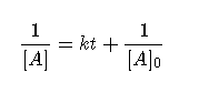
For these second-order reactions, the integrated rate law is:

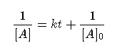
where the terms in the equation have their usual meanings as defined earlier.

The integrated rate law for our second-order reactions has the form of the equation of a straight line:

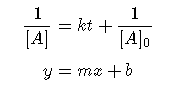
A plot of 1[A] versus t for a second-order reaction is a straight line with a slope of k and an intercept of 1[A]0. If the plot is not a straight line, then the reaction is not second order.

Zero-Order Reactions

For zero-order reactions, the differential rate law is:

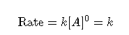
A zero-order reaction thus exhibits a constant reaction rate, regardless of the concentration of its reactants.

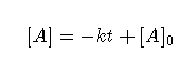
The integrated rate law for a zero-order reaction also has the form of the equation of a straight line:

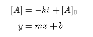
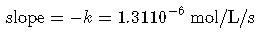
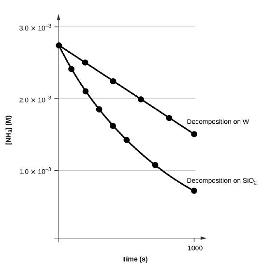
A plot of [A] versus t$t$ for a zero-order reaction is a straight line with a slope of −k and an intercept of [A]0. Figure $3$ shows a plot of [NH3] versus t for the decomposition of ammonia on a hot tungsten wire and for the decomposition of ammonia on hot quartz (SiO2). The decomposition of NH3 on hot tungsten is zero order; the plot is a straight line. The decomposition of NH3 on hot quartz is not zero order (it is first order). From the slope of the line for the zero-order decomposition, we can determine the rate constant:

The Half-Life of a Reaction

The half-life of a reaction (t1/2) is the time required for one-half of a given amount of reactant to be consumed. In each succeeding half-life, half of the remaining concentration of the reactant is consumed. Using the decomposition of hydrogen peroxide as an example, we find that during the first half-life (from 0.00 hours to 6.00 hours), the concentration of H2O2 decreases from 1.000 M to 0.500 M. During the second half-life (from 6.00 hours to 12.00 hours), it decreases from 0.500 M to 0.250 M; during the third half-life, it decreases from 0.250 M to 0.125 M. The concentration of H2O2 decreases by half during each successive period of 6.00 hours. The decomposition of hydrogen peroxide is a first-order reaction, and, as can be shown, the half-life of a first-order reaction is independent of the concentration of the reactant. However, half-lives of reactions with other orders depend on the concentrations of the reactants.

First-Order Reactions

We can derive an equation for determining the half-life of a first-order reaction from the alternate form of the integrated rate law as follows:

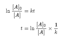
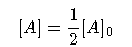
If we set the time t equal to the half-life, t1/2, the corresponding concentration of A at this time is equal to one-half of its initial concentration. Hence, when t=t1/2, [A]=12[A]0.

Therefore:

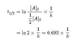
Thus:

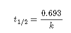
the rate constant k. A fast reaction (shorter half-life) will have a larger k; a slow reaction (longer half-life) will have a smaller k.

Second-Order Reactions

We can derive the equation for calculating the half-life of a second order as follows:

or

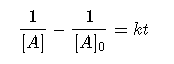
If

then

and we can write:

Thus:

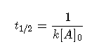
For a second-order reaction, t1/2 is inversely proportional to the concentration of the reactant, and the half-life increases as the reaction proceeds because the concentration of reactant decreases. Consequently, we find the use of the half-life concept to be more complex for second-order reactions than for first-order reactions. Unlike with first-order reactions, the rate constant of a second-order reaction cannot be calculated directly from the half-life unless the initial concentration is known.

Zero-Order Reactions

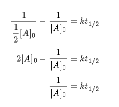
We can derive an equation for calculating the half-life of a zero order reaction as follows:

When half of the initial amount of reactant has been consumed 

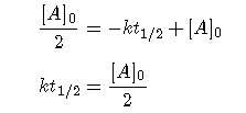
and

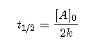
The half-life of a zero-order reaction increases as the initial concentration increases. Equations for both differential and integrated rate laws and the corresponding half-lives for zero-, first-, and second-order reactions are summarized in Table $1$.

Table $1$: Summary of Rate Laws for Zero-, First-, and Second-Order Reactions

	Zero-Order	First-Order	Second-Order
rate law	rate = k	rate = k[A]	rate = k[A]2
units of rate constant	M s−1	s−1	M−1 s−1
integrated rate law	[A] = −kt + [A]0	ln[A] = −kt + ln[A]0	1[A]=kt+(1[A]0)
plot needed for linear fit of rate data	[A] vs. t	ln[A] vs. t	1[A]${\displaystyle \frac{1}{[A]}}$ vs. t
relationship between slope of linear plot and rate constant	k = −slope	k = −slope	k = +slope
half-life	t1/2=[A]02k	t1/2=0.693k	t1/2=1[A]0k

Summary

Differential rate laws can be determined by the method of initial rates or other methods. We measure values for the initial rates of a reaction at different concentrations of the reactants. From these measurements, we determine the order of the reaction in each reactant. Integrated rate laws are determined by integration of the corresponding differential rate laws. Rate constants for those rate laws are determined from measurements of concentration at various times during a reaction.

The half-life of a reaction is the time required to decrease the amount of a given reactant by one-half. The half-life of a zero-order reaction decreases as the initial concentration of the reactant in the reaction decreases. The half-life of a first-order reaction is independent of concentration, and the half-life of a second-order reaction decreases as the concentration increases.