python图片处理技术
python数字图像处理(8):对比度与亮度调整
图像亮度与对比度的调整,是放在skimage包的exposure模块里面
1、gamma调整
原理:I=Ig
对原图像的像素,进行幂运算,得到新的像素值。公式中的g就是gamma值。
如果gamma>1, 新图像比原图像暗
如果gamma<1,新图像比原图像亮
函数格式为:skimage.exposure.adjust_gamma(image, gamma=1)
gamma参数默认为1,原像不发生变化 。

from skimage import data, exposure, img_as_float
import matplotlib.pyplot as plt
image = img_as_float(data.moon())
gam1= exposure.adjust_gamma(image, 2)   #调暗
gam2= exposure.adjust_gamma(image, 0.5)  #调亮
plt.figure('adjust_gamma',figsize=(8,8))

plt.subplot(131)
plt.title('origin image')
plt.imshow(image,plt.cm.gray)
plt.axis('off')

plt.subplot(132)
plt.title('gamma=2')
plt.imshow(gam1,plt.cm.gray)
plt.axis('off')

plt.subplot(133)
plt.title('gamma=0.5')
plt.imshow(gam2,plt.cm.gray)
plt.axis('off')

plt.show()

2、log对数调整
这个刚好和gamma相反
原理:I=log(I)
from skimage import data, exposure, img_as_float
import matplotlib.pyplot as plt
image = img_as_float(data.moon())
gam1= exposure.adjust_log(image)   #对数调整
plt.figure('adjust_gamma',figsize=(8,8))

plt.subplot(121)
plt.title('origin image')
plt.imshow(image,plt.cm.gray)
plt.axis('off')

plt.subplot(122)
plt.title('log')
plt.imshow(gam1,plt.cm.gray)
plt.axis('off')

plt.show()

3、判断图像对比度是否偏低
函数:is_low_contrast(img)
返回一个bool型值
from skimage import data, exposure
image =data.moon()
result=exposure.is_low_contrast(image)
print(result)
输出为False
4、调整强度
函数:skimage.exposure.rescale_intensity(image, in_range='image', out_range='dtype')
in_range 表示输入图片的强度范围,默认为'image', 表示用图像的最大/最小像素值作为范围
out_range 表示输出图片的强度范围,默认为'dype', 表示用图像的类型的最大/最小值作为范围
默认情况下,输入图片的[min,max]范围被拉伸到[dtype.min, dtype.max],如果dtype=uint8, 那么dtype.min=0, dtype.max=255
import numpy as np
from skimage import exposure
image = np.array([51, 102, 153], dtype=np.uint8)
mat=exposure.rescale_intensity(image)
print(mat)
输出为[ 0 127 255]
即像素最小值由51变为0,最大值由153变为255,整体进行了拉伸,但是数据类型没有变,还是uint8
前面我们讲过,可以通过img_as_float()函数将unit8类型转换为float型,实际上还有更简单的方法,就是乘以1.0
import numpy as np
image = np.array([51, 102, 153], dtype=np.uint8)
print(image*1.0)
即由[51,102,153]变成了[ 51. 102. 153.]
而float类型的范围是[0,1],因此对float进行rescale_intensity 调整后,范围变为[0,1],而不是[0,255]
import numpy as np
from skimage import exposure
image = np.array([51, 102, 153], dtype=np.uint8)
tmp=image*1.0
mat=exposure.rescale_intensity(tmp)
print(mat)
结果为[ 0. 0.5 1. ]
如果原始像素值不想被拉伸,只是等比例缩小,就使用in_range参数,如:
import numpy as np
from skimage import exposure
image = np.array([51, 102, 153], dtype=np.uint8)
tmp=image*1.0
mat=exposure.rescale_intensity(tmp,in_range=(0,255))
print(mat)
输出为:[ 0.2 0.4 0.6],即原像素值除以255
如果参数in_range的[main,max]范围要比原始像素值的范围[min,max] 大或者小,那就进行裁剪,如:
mat=exposure.rescale_intensity(tmp,in_range=(0,102))
print(mat)
输出[ 0.5 1. 1. ],即原像素值除以102,超出1的变为1
如果一个数组里面有负数,现在想调整到正数,就使用out_range参数。如:
import numpy as np
from skimage import exposure
image = np.array([-10, 0, 10], dtype=np.int8)
mat=exposure.rescale_intensity(image, out_range=(0, 127))
print(mat)
输出[ 0 63 127]
python数字图像处理(9):直方图与均衡化
在图像处理中,直方图是非常重要,也是非常有用的一个处理要素。
在skimage库中对直方图的处理,是放在exposure这个模块中。
1、计算直方图
函数:skimage.exposure.histogram(image, nbins=256)
在numpy包中,也提供了一个计算直方图的函数histogram(),两者大同小义。
返回一个tuple(hist, bins_center), 前一个数组是直方图的统计量,后一个数组是每个bin的中间值
import numpy as np
from skimage import exposure,data
image =data.camera()*1.0
hist1=np.histogram(image, bins=2)   #用numpy包计算直方图
hist2=exposure.histogram(image, nbins=2)  #用skimage计算直方图
print(hist1)
print(hist2)
输出:
(array([107432, 154712], dtype=int64), array([ 0. , 127.5, 255. ]))
(array([107432, 154712], dtype=int64), array([ 63.75, 191.25]))
分成两个bin,每个bin的统计量是一样的,但numpy返回的是每个bin的两端的范围值,而skimage返回的是每个bin的中间值
2、绘制直方图
绘图都可以调用matplotlib.pyplot库来进行,其中的hist函数可以直接绘制直方图。
调用方式:
n, bins, patches = plt.hist(arr, bins=10, normed=0, facecolor='black', edgecolor='black',alpha=1,histtype='bar')
hist的参数非常多,但常用的就这六个,只有第一个是必须的,后面四个可选
arr: 需要计算直方图的一维数组
bins: 直方图的柱数,可选项,默认为10
normed: 是否将得到的直方图向量归一化。默认为0
facecolor: 直方图颜色
edgecolor: 直方图边框颜色
alpha: 透明度
histtype: 直方图类型,‘bar’, ‘barstacked’, ‘step’, ‘stepfilled’
返回值 :
n: 直方图向量,是否归一化由参数normed设定
bins: 返回各个bin的区间范围
patches: 返回每个bin里面包含的数据,是一个list
from skimage import data
import matplotlib.pyplot as plt
img=data.camera()
plt.figure("hist")
arr=img.flatten()
n, bins, patches = plt.hist(arr, bins=256, normed=1,edgecolor='None',facecolor='red')
plt.show()

其中的flatten()函数是numpy包里面的,用于将二维数组序列化成一维数组。
是按行序列,如
mat=[[1 2 3
4 5 6]]
经过 mat.flatten()后,就变成了
mat=[1 2 3 4 5 6]
3、彩色图片三通道直方图
一般来说直方图都是征对灰度图的,如果要画rgb图像的三通道直方图,实际上就是三个直方图的叠加。
from skimage import data
import matplotlib.pyplot as plt
img=data.lena()
ar=img[:,:,0].flatten()
plt.hist(ar, bins=256, normed=1,facecolor='r',edgecolor='r',hold=1)
ag=img[:,:,1].flatten()
plt.hist(ag, bins=256, normed=1, facecolor='g',edgecolor='g',hold=1)
ab=img[:,:,2].flatten()
plt.hist(ab, bins=256, normed=1, facecolor='b',edgecolor='b')
plt.show()
其中,加一个参数hold=1,表示可以叠加

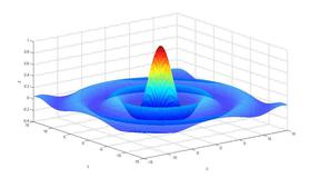
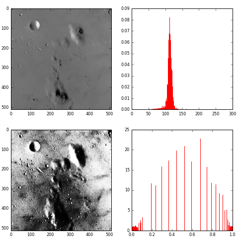
4、直方图均衡化
如果一副图像的像素占有很多的灰度级而且分布均匀,那么这样的图像往往有高对比度和多变的灰度色调。直方图均衡化就是一种能仅靠输入图像直方图信息自动达到这种效果的变换函数。它的基本思想是对图像中像素个数多的灰度级进行展宽,而对图像中像素个数少的灰度进行压缩,从而扩展取值的动态范围,提高了对比度和灰度色调的变化,使图像更加清晰。
from skimage import data,exposure
import matplotlib.pyplot as plt
img=data.moon()
plt.figure("hist",figsize=(8,8))

arr=img.flatten()
plt.subplot(221)
plt.imshow(img,plt.cm.gray)  #原始图像
plt.subplot(222)
plt.hist(arr, bins=256, normed=1,edgecolor='None',facecolor='red') #原始图像直方图

img1=exposure.equalize_hist(img)
arr1=img1.flatten()
plt.subplot(223)
plt.imshow(img1,plt.cm.gray)  #均衡化图像
plt.subplot(224)
plt.hist(arr1, bins=256, normed=1,edgecolor='None',facecolor='red') #均衡化直方图

plt.show()
python数字图像处理(10):图像简单滤波
对图像进行滤波,可以有两种效果:一种是平滑滤波,用来抑制噪声;另一种是微分算子,可以用来检测边缘和特征提取。
skimage库中通过filters模块进行滤波操作。
1、sobel算子
sobel算子可用来检测边缘
函数格式为:skimage.filters.sobel(image, mask=None)
from skimage import data,filters
import matplotlib.pyplot as plt
img = data.camera()
edges = filters.sobel(img)
plt.imshow(edges,plt.cm.gray)

2、roberts算子
roberts算子和sobel算子一样,用于检测边缘
调用格式也是一样的:
edges = filters.roberts(img)
3、scharr算子
功能同sobel,调用格式:
edges = filters.scharr(img)
4、prewitt算子
功能同sobel,调用格式:
edges = filters.prewitt(img)
5、canny算子
canny算子也是用于提取边缘特征,但它不是放在filters模块,而是放在feature模块
函数格式:skimage.feature.canny(image,sigma=1.0)
可以修改sigma的值来调整效果
from skimage import data,filters,feature
import matplotlib.pyplot as plt
img = data.camera()
edges1 = feature.canny(img)   #sigma=1
edges2 = feature.canny(img,sigma=3)   #sigma=3

plt.figure('canny',figsize=(8,8))
plt.subplot(121)
plt.imshow(edges1,plt.cm.gray)

plt.subplot(122)
plt.imshow(edges2,plt.cm.gray)

plt.show()

从结果可以看出,sigma越小,边缘线条越细小。
6、gabor滤波
gabor滤波可用来进行边缘检测和纹理特征提取。
函数调用格式:skimage.filters.gabor_filter(image, frequency)
通过修改frequency值来调整滤波效果,返回一对边缘结果,一个是用真实滤波核的滤波结果,一个是想象的滤波核的滤波结果。
from skimage import data,filters
import matplotlib.pyplot as plt
img = data.camera()
filt_real, filt_imag = filters.gabor_filter(img,frequency=0.6)

plt.figure('gabor',figsize=(8,8))

plt.subplot(121)
plt.title('filt_real')
plt.imshow(filt_real,plt.cm.gray)

plt.subplot(122)
plt.title('filt-imag')
plt.imshow(filt_imag,plt.cm.gray)

plt.show()

以上为frequency=0.6的结果图。

以上为frequency=0.1的结果图
7、gaussian滤波
多维的滤波器,是一种平滑滤波,可以消除高斯噪声。
调用函数为:skimage.filters.gaussian_filter(image, sigma)
通过调节sigma的值来调整滤波效果
from skimage import data,filters
import matplotlib.pyplot as plt
img = data.astronaut()
edges1 = filters.gaussian_filter(img,sigma=0.4)   #sigma=0.4
edges2 = filters.gaussian_filter(img,sigma=5)   #sigma=5

plt.figure('gaussian',figsize=(8,8))
plt.subplot(121)
plt.imshow(edges1,plt.cm.gray)

plt.subplot(122)
plt.imshow(edges2,plt.cm.gray)

plt.show()

可见sigma越大,过滤后的图像越模糊
8.median
中值滤波,一种平滑滤波,可以消除噪声。
需要用skimage.morphology模块来设置滤波器的形状。
from skimage import data,filters
import matplotlib.pyplot as plt
from skimage.morphology import disk
img = data.camera()
edges1 = filters.median(img,disk(5))
edges2= filters.median(img,disk(9))

plt.figure('median',figsize=(8,8))

plt.subplot(121)
plt.imshow(edges1,plt.cm.gray)

plt.subplot(122)
plt.imshow(edges2,plt.cm.gray)

plt.show()

从结果可以看出,滤波器越大,图像越模糊。
9、水平、垂直边缘检测
上边所举的例子都是进行全部边缘检测,有些时候我们只需要检测水平边缘,或垂直边缘,就可用下面的方法。
水平边缘检测:sobel_h, prewitt_h, scharr_h
垂直边缘检测: sobel_v, prewitt_v, scharr_v
from skimage import data,filters
import matplotlib.pyplot as plt
img = data.camera()
edges1 = filters.sobel_h(img)
edges2 = filters.sobel_v(img)

plt.figure('sobel_v_h',figsize=(8,8))

plt.subplot(121)
plt.imshow(edges1,plt.cm.gray)

plt.subplot(122)
plt.imshow(edges2,plt.cm.gray)

plt.show()

上边左图为检测出的水平边缘,右图为检测出的垂直边缘。
10、交叉边缘检测
可使用Roberts的十字交叉核来进行过滤,以达到检测交叉边缘的目的。这些交叉边缘实际上是梯度在某个方向上的一个分量。
其中一个核:
 0   1
-1   0
对应的函数:
roberts_neg_diag(image)
例:
from skimage import data,filters
import matplotlib.pyplot as plt
img =data.camera()
dst =filters.roberts_neg_diag(img)

plt.figure('filters',figsize=(8,8))
plt.subplot(121)
plt.title('origin image')
plt.imshow(img,plt.cm.gray)

plt.subplot(122)
plt.title('filted image')
plt.imshow(dst,plt.cm.gray)

另外一个核:
1   0
0  -1
对应函数为:
roberts_pos_diag(image)
from skimage import data,filters
import matplotlib.pyplot as plt
img =data.camera()
dst =filters.roberts_pos_diag(img)

plt.figure('filters',figsize=(8,8))
plt.subplot(121)
plt.title('origin image')
plt.imshow(img,plt.cm.gray)

plt.subplot(122)
plt.title('filted image')
plt.imshow(dst,plt.cm.gray)

python数字图像处理(11):图像自动阈值分割
图像阈值分割是一种广泛应用的分割技术,利用图像中要提取的目标区域与其背景在灰度特性上的差异,把图像看作具有不同灰度级的两类区域(目标区域和背景区域)的组合,选取一个比较合理的阈值,以确定图像中每个像素点应该属于目标区域还是背景区域,从而产生相应的二值图像。
在skimage库中,阈值分割的功能是放在filters模块中。
我们可以手动指定一个阈值,从而来实现分割。也可以让系统自动生成一个阈值,下面几种方法就是用来自动生成阈值。
1、threshold_otsu
基于Otsu的阈值分割方法,函数调用格式:
skimage.filters.threshold_otsu(image, nbins=256)
参数image是指灰度图像,返回一个阈值。
from skimage import data,filters
import matplotlib.pyplot as plt
image = data.camera()
thresh = filters.threshold_otsu(image)   #返回一个阈值
dst =(image <= thresh)*1.0   #根据阈值进行分割

plt.figure('thresh',figsize=(8,8))

plt.subplot(121)
plt.title('original image')
plt.imshow(image,plt.cm.gray)

plt.subplot(122)
plt.title('binary image')
plt.imshow(dst,plt.cm.gray)

plt.show()
返回阈值为87,根据87进行分割得下图:

2、threshold_yen
使用方法同上:
thresh = filters.threshold_yen(image)
返回阈值为198,分割如下图:

3、threshold_li
使用方法同上:
thresh = filters.threshold_li(image)
返回阈值64.5,分割如下图:

4、threshold_isodata
阈值计算方法:
threshold = (image[image <= threshold].mean() +image[image > threshold].mean()) / 2.0
使用方法同上:
thresh = filters.threshold_isodata(image)
返回阈值为87,因此分割效果和threshold_otsu一样。
5、threshold_adaptive
调用函数为:
skimage.filters.threshold_adaptive(image, block_size, method='gaussian')
block_size: 块大小,指当前像素的相邻区域大小,一般是奇数(如3,5,7。。。)
method: 用来确定自适应阈值的方法,有'mean', 'generic', 'gaussian' 和 'median'。省略时默认为gaussian
该函数直接访问一个阈值后的图像,而不是阈值。
from skimage import data,filters
import matplotlib.pyplot as plt
image = data.camera()
dst =filters.threshold_adaptive(image, 15) #返回一个阈值图像

plt.figure('thresh',figsize=(8,8))

plt.subplot(121)
plt.title('original image')
plt.imshow(image,plt.cm.gray)

plt.subplot(122)
plt.title('binary image')
plt.imshow(dst,plt.cm.gray)

plt.show()

大家可以修改block_size的大小和method值来查看更多的效果。如:
dst1 =filters.threshold_adaptive(image,31,'mean')
dst2 =filters.threshold_adaptive(image,5,'median')
两种效果如下:

python数字图像处理(12):基本图形的绘制
图形包括线条、圆形、椭圆形、多边形等。
在skimage包中,绘制图形用的是draw模块,不要和绘制图像搞混了。
1、画线条
函数调用格式为:
skimage.draw.line(r1,c1,r2,c2)
r1,r2: 开始点的行数和结束点的行数
c1,c2: 开始点的列数和结束点的列数
返回当前绘制图形上所有点的坐标,如:
rr, cc =draw.line(1, 5, 8, 2)
表示从(1,5)到(8,2)连一条线,返回线上所有的像素点坐标[rr,cc]
from skimage import draw,data
import matplotlib.pyplot as plt
img=data.chelsea()
rr, cc =draw.line(1, 150, 470, 450)
img[rr, cc] =255
plt.imshow(img,plt.cm.gray)

如果想画其它颜色的线条,则可以使用set_color()函数,格式为:
skimage.draw.set_color(img, coords, color)
例:
draw.set_color(img,[rr,cc],[255,0,0])
则绘制红色线条。
from skimage import draw,data
import matplotlib.pyplot as plt
img=data.chelsea()
rr, cc =draw.line(1, 150, 270, 250)
draw.set_color(img,[rr,cc],[0,0,255])
plt.imshow(img,plt.cm.gray)

2、画圆
函数格式:skimage.draw.circle(cy, cx, radius)
cy和cx表示圆心点,radius表示半径
from skimage import draw,data
import matplotlib.pyplot as plt
img=data.chelsea()
rr, cc=draw.circle(150,150,50)
draw.set_color(img,[rr,cc],[255,0,0])
plt.imshow(img,plt.cm.gray)

3、多边形
函数格式:skimage.draw.polygon(Y,X)
Y为多边形顶点的行集合,X为各顶点的列值集合。
from skimage import draw,data
import matplotlib.pyplot as plt
import numpy as np
img=data.chelsea()
Y=np.array([10,10,60,60])
X=np.array([200,400,400,200])
rr, cc=draw.polygon(Y,X)
draw.set_color(img,[rr,cc],[255,0,0])
plt.imshow(img,plt.cm.gray)

我在此处只设置了四个顶点,因此是个四边形。
4、椭圆
格式:skimage.draw.ellipse(cy, cx, yradius, xradius)
cy和cx为中心点坐标,yradius和xradius代表长短轴。
from skimage import draw,data
import matplotlib.pyplot as plt
img=data.chelsea()
rr, cc=draw.ellipse(150, 150, 30, 80)
draw.set_color(img,[rr,cc],[255,0,0])
plt.imshow(img,plt.cm.gray)

5、贝塞儿曲线
格式:skimage.draw.bezier_curve(y1,x1,y2,x2,y3,x3,weight)
y1,x1表示第一个控制点坐标
y2,x2表示第二个控制点坐标
y3,x3表示第三个控制点坐标
weight表示中间控制点的权重,用于控制曲线的弯曲度。
from skimage import draw,data
import matplotlib.pyplot as plt
img=data.chelsea()
rr, cc=draw.bezier_curve(150,50,50,280,260,400,2)
draw.set_color(img,[rr,cc],[255,0,0])
plt.imshow(img,plt.cm.gray)

6、画空心圆
和前面的画圆是一样的,只是前面是实心圆,而此处画空心圆,只有边框线。
格式:skimage.draw.circle_perimeter(yx,yc,radius)
yx,yc是圆心坐标,radius是半径
from skimage import draw,data
import matplotlib.pyplot as plt
img=data.chelsea()
rr, cc=draw.circle_perimeter(150,150,50)
draw.set_color(img,[rr,cc],[255,0,0])
plt.imshow(img,plt.cm.gray)

7、空心椭圆
格式:skimage.draw.ellipse_perimeter(cy, cx, yradius, xradius)
cy,cx表示圆心
yradius,xradius表示长短轴
from skimage import draw,data
import matplotlib.pyplot as plt
img=data.chelsea()
rr, cc=draw.ellipse_perimeter(150, 150, 30, 80)
draw.set_color(img,[rr,cc],[255,0,0])
plt.imshow(img,plt.cm.gray)

python数字图像处理(13):基本形态学滤波
对图像进行形态学变换。变换对象一般为灰度图或二值图,功能函数放在morphology子模块内。
1、膨胀(dilation)
原理:一般对二值图像进行操作。找到像素值为1的点,将它的邻近像素点都设置成这个值。1值表示白,0值表示黑,因此膨胀操作可以扩大白色值范围,压缩黑色值范围。一般用来扩充边缘或填充小的孔洞。
功能函数:skimage.morphology.dilation(image, selem=None)
selem表示结构元素,用于设定局部区域的形状和大小。
from skimage import data
import skimage.morphology as sm
import matplotlib.pyplot as plt
img=data.checkerboard()
dst1=sm.dilation(img,sm.square(5))  #用边长为5的正方形滤波器进行膨胀滤波
dst2=sm.dilation(img,sm.square(15))  #用边长为15的正方形滤波器进行膨胀滤波

plt.figure('morphology',figsize=(8,8))
plt.subplot(131)
plt.title('origin image')
plt.imshow(img,plt.cm.gray)

plt.subplot(132)
plt.title('morphological image')
plt.imshow(dst1,plt.cm.gray)

plt.subplot(133)
plt.title('morphological image')
plt.imshow(dst2,plt.cm.gray)
分别用边长为5或15的正方形滤波器对棋盘图片进行膨胀操作,结果如下:

可见滤波器的大小,对操作结果的影响非常大。一般设置为奇数。
除了正方形的滤波器外,滤波器的形状还有一些,现列举如下:
morphology.square: 正方形
morphology.disk: 平面圆形
morphology.ball: 球形
morphology.cube: 立方体形
morphology.diamond: 钻石形
morphology.rectangle: 矩形
morphology.star: 星形
morphology.octagon: 八角形
morphology.octahedron: 八面体
注意,如果处理图像为二值图像(只有0和1两个值),则可以调用:
skimage.morphology.binary_dilation(image, selem=None)
用此函数比处理灰度图像要快。
2、腐蚀(erosion)
函数:skimage.morphology.erosion(image, selem=None)
selem表示结构元素,用于设定局部区域的形状和大小。
和膨胀相反的操作,将0值扩充到邻近像素。扩大黑色部分,减小白色部分。可用来提取骨干信息,去掉毛刺,去掉孤立的像素。
from skimage import data
import skimage.morphology as sm
import matplotlib.pyplot as plt
img=data.checkerboard()
dst1=sm.erosion(img,sm.square(5))  #用边长为5的正方形滤波器进行膨胀滤波
dst2=sm.erosion(img,sm.square(25))  #用边长为25的正方形滤波器进行膨胀滤波

plt.figure('morphology',figsize=(8,8))
plt.subplot(131)
plt.title('origin image')
plt.imshow(img,plt.cm.gray)

plt.subplot(132)
plt.title('morphological image')
plt.imshow(dst1,plt.cm.gray)

plt.subplot(133)
plt.title('morphological image')
plt.imshow(dst2,plt.cm.gray)

注意,如果处理图像为二值图像(只有0和1两个值),则可以调用:
skimage.morphology.binary_erosion(image, selem=None)
用此函数比处理灰度图像要快。
3、开运算(opening)
函数:skimage.morphology.openning(image, selem=None)
selem表示结构元素,用于设定局部区域的形状和大小。
先腐蚀再膨胀,可以消除小物体或小斑块。
from skimage import io,color
import skimage.morphology as sm
import matplotlib.pyplot as plt
img=color.rgb2gray(io.imread('d:/pic/mor.png'))
dst=sm.opening(img,sm.disk(9))  #用边长为9的圆形滤波器进行膨胀滤波

plt.figure('morphology',figsize=(8,8))
plt.subplot(121)
plt.title('origin image')
plt.imshow(img,plt.cm.gray)
plt.axis('off')

plt.subplot(122)
plt.title('morphological image')
plt.imshow(dst,plt.cm.gray)
plt.axis('off')

注意,如果处理图像为二值图像(只有0和1两个值),则可以调用:
skimage.morphology.binary_opening(image, selem=None)
用此函数比处理灰度图像要快。
4、闭运算(closing)
函数:skimage.morphology.closing(image, selem=None)
selem表示结构元素,用于设定局部区域的形状和大小。
先膨胀再腐蚀,可用来填充孔洞。
from skimage import io,color
import skimage.morphology as sm
import matplotlib.pyplot as plt
img=color.rgb2gray(io.imread('d:/pic/mor.png'))
dst=sm.closing(img,sm.disk(9))  #用边长为5的圆形滤波器进行膨胀滤波

plt.figure('morphology',figsize=(8,8))
plt.subplot(121)
plt.title('origin image')
plt.imshow(img,plt.cm.gray)
plt.axis('off')

plt.subplot(122)
plt.title('morphological image')
plt.imshow(dst,plt.cm.gray)
plt.axis('off')

注意,如果处理图像为二值图像(只有0和1两个值),则可以调用:
skimage.morphology.binary_closing(image, selem=None)
用此函数比处理灰度图像要快。
5、白帽(white-tophat)
函数:skimage.morphology.white_tophat(image, selem=None)
selem表示结构元素,用于设定局部区域的形状和大小。
将原图像减去它的开运算值,返回比结构化元素小的白点
from skimage import io,color
import skimage.morphology as sm
import matplotlib.pyplot as plt
img=color.rgb2gray(io.imread('d:/pic/mor.png'))
dst=sm.white_tophat(img,sm.square(21))

plt.figure('morphology',figsize=(8,8))
plt.subplot(121)
plt.title('origin image')
plt.imshow(img,plt.cm.gray)
plt.axis('off')

plt.subplot(122)
plt.title('morphological image')
plt.imshow(dst,plt.cm.gray)
plt.axis('off')

6、黑帽(black-tophat)
函数:skimage.morphology.black_tophat(image, selem=None)
selem表示结构元素,用于设定局部区域的形状和大小。
将原图像减去它的闭运算值,返回比结构化元素小的黑点,且将这些黑点反色。
from skimage import io,color
import skimage.morphology as sm
import matplotlib.pyplot as plt
img=color.rgb2gray(io.imread('d:/pic/mor.png'))
dst=sm.black_tophat(img,sm.square(21))

plt.figure('morphology',figsize=(8,8))
plt.subplot(121)
plt.title('origin image')
plt.imshow(img,plt.cm.gray)
plt.axis('off')

plt.subplot(122)
plt.title('morphological image')
plt.imshow(dst,plt.cm.gray)
plt.axis('off')

python数字图像处理(14):高级滤波
本文提供更多更强大的滤波方法,这些方法放在filters.rank子模块内。
这些方法需要用户自己设定滤波器的形状和大小,因此需要导入morphology模块来设定。
1、autolevel
这个词在photoshop里面翻译成自动色阶,用局部直方图来对图片进行滤波分级。
该滤波器局部地拉伸灰度像素值的直方图,以覆盖整个像素值范围。
格式:skimage.filters.rank.autolevel(image, selem)
selem表示结构化元素,用于设定滤波器。
from skimage import data,color
import matplotlib.pyplot as plt
from skimage.morphology import disk
import skimage.filters.rank as sfr
img =color.rgb2gray(data.lena())
auto =sfr.autolevel(img, disk(5))  #半径为5的圆形滤波器

plt.figure('filters',figsize=(8,8))
plt.subplot(121)
plt.title('origin image')
plt.imshow(img,plt.cm.gray)

plt.subplot(122)
plt.title('filted image')
plt.imshow(auto,plt.cm.gray)

2、bottomhat 与 tophat
bottomhat: 此滤波器先计算图像的形态学闭运算,然后用原图像减去运算的结果值,有点像黑帽操作。
bottomhat: 此滤波器先计算图像的形态学开运算,然后用原图像减去运算的结果值,有点像白帽操作。
格式:
skimage.filters.rank.bottomhat(image, selem)
skimage.filters.rank.tophat(image, selem)
selem表示结构化元素,用于设定滤波器。
下面是bottomhat滤波的例子:
from skimage import data,color
import matplotlib.pyplot as plt
from skimage.morphology import disk
import skimage.filters.rank as sfr
img =color.rgb2gray(data.lena())
auto =sfr.bottomhat(img, disk(5))  #半径为5的圆形滤波器

plt.figure('filters',figsize=(8,8))
plt.subplot(121)
plt.title('origin image')
plt.imshow(img,plt.cm.gray)

plt.subplot(122)
plt.title('filted image')
plt.imshow(auto,plt.cm.gray)

3、enhance_contrast
对比度增强。求出局部区域的最大值和最小值,然后看当前点像素值最接近最大值还是最小值,然后替换为最大值或最小值。
函数: enhance_contrast(image, selem)
selem表示结构化元素,用于设定滤波器。
from skimage import data,color
import matplotlib.pyplot as plt
from skimage.morphology import disk
import skimage.filters.rank as sfr
img =color.rgb2gray(data.lena())
auto =sfr.enhance_contrast(img, disk(5))  #半径为5的圆形滤波器

plt.figure('filters',figsize=(8,8))
plt.subplot(121)
plt.title('origin image')
plt.imshow(img,plt.cm.gray)

plt.subplot(122)
plt.title('filted image')
plt.imshow(auto,plt.cm.gray)

4、entropy
求局部熵,熵是使用基为2的对数运算出来的。该函数将局部区域的灰度值分布进行二进制编码,返回编码的最小值。
函数格式:entropy(image, selem)
selem表示结构化元素,用于设定滤波器。
from skimage import data,color
import matplotlib.pyplot as plt
from skimage.morphology import disk
import skimage.filters.rank as sfr
img =color.rgb2gray(data.lena())
dst =sfr.entropy(img, disk(5))  #半径为5的圆形滤波器

plt.figure('filters',figsize=(8,8))
plt.subplot(121)
plt.title('origin image')
plt.imshow(img,plt.cm.gray)

plt.subplot(122)
plt.title('filted image')
plt.imshow(dst,plt.cm.gray)

5、equalize
均衡化滤波。利用局部直方图对图像进行均衡化滤波。
函数格式:equalize(image, selem)
selem表示结构化元素,用于设定滤波器。
from skimage import data,color
import matplotlib.pyplot as plt
from skimage.morphology import disk
import skimage.filters.rank as sfr
img =color.rgb2gray(data.lena())
dst =sfr.equalize(img, disk(5))  #半径为5的圆形滤波器

plt.figure('filters',figsize=(8,8))
plt.subplot(121)
plt.title('origin image')
plt.imshow(img,plt.cm.gray)

plt.subplot(122)
plt.title('filted image')
plt.imshow(dst,plt.cm.gray)

6、gradient
返回图像的局部梯度值(如:最大值-最小值),用此梯度值代替区域内所有像素值。
函数格式:gradient(image, selem)
selem表示结构化元素,用于设定滤波器。
from skimage import data,color
import matplotlib.pyplot as plt
from skimage.morphology import disk
import skimage.filters.rank as sfr
img =color.rgb2gray(data.lena())
dst =sfr.gradient(img, disk(5))  #半径为5的圆形滤波器

plt.figure('filters',figsize=(8,8))
plt.subplot(121)
plt.title('origin image')
plt.imshow(img,plt.cm.gray)

plt.subplot(122)
plt.title('filted image')
plt.imshow(dst,plt.cm.gray)

7、其它滤波器
滤波方式很多,下面不再一一详细讲解,仅给出核心代码,所有的函数调用方式都是一样的。
最大值滤波器(maximum):返回图像局部区域的最大值,用此最大值代替该区域内所有像素值。
dst =sfr.maximum(img, disk(5))
最小值滤波器(minimum):返回图像局部区域内的最小值,用此最小值取代该区域内所有像素值。
dst =sfr.minimum(img, disk(5))
均值滤波器(mean) : 返回图像局部区域内的均值,用此均值取代该区域内所有像素值。
dst =sfr.mean(img, disk(5))
中值滤波器(median): 返回图像局部区域内的中值,用此中值取代该区域内所有像素值。
dst =sfr.median(img, disk(5))
莫代尔滤波器(modal) : 返回图像局部区域内的modal值,用此值取代该区域内所有像素值。
dst =sfr.modal(img, disk(5))
otsu阈值滤波(otsu): 返回图像局部区域内的otsu阈值,用此值取代该区域内所有像素值。
dst =sfr.otsu(img, disk(5))
阈值滤波(threshhold): 将图像局部区域中的每个像素值与均值比较,大于则赋值为1,小于赋值为0,得到一个二值图像。
dst =sfr.threshold(img, disk(5))
减均值滤波(subtract_mean): 将局部区域中的每一个像素,减去该区域中的均值。
dst =sfr.subtract_mean(img, disk(5))
求和滤波(sum) :求局部区域的像素总和,用此值取代该区域内所有像素值。
dst =sfr.sum(img, disk(5))
python数字图像处理(15):霍夫线变换
在图片处理中,霍夫变换主要是用来检测图片中的几何形状,包括直线、圆、椭圆等。
在skimage中,霍夫变换是放在tranform模块内,本篇主要讲解霍夫线变换。
对于平面中的一条直线,在笛卡尔坐标系中,可用y=mx+b来表示,其中m为斜率,b为截距。但是如果直线是一条垂直线,则m为无穷大,所有通常我们在另一坐标系中表示直线,即极坐标系下的r=xcos(theta)+ysin(theta)。即可用(r,theta)来表示一条直线。其中r为该直线到原点的距离,theta为该直线的垂线与x轴的夹角。如下图所示。
对于一个给定的点(x0,y0), 我们在极坐标下绘出所有通过它的直线(r,theta),将得到一条正弦曲线。如果将图片中的所有非0点的正弦曲线都绘制出来,则会存在一些交点。所有经过这个交点的正弦曲线,说明都拥有同样的(r,theta), 意味着这些点在一条直线上。
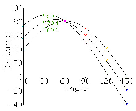
发上图所示,三个点(对应图中的三条正弦曲线)在一条直线上,因为这三个曲线交于一点,具有相同的(r, theta)。霍夫线变换就是利用这种方法来寻找图中的直线。
函数:skimage.transform.hough_line(img)
返回三个值:
h: 霍夫变换累积器
theta: 点与x轴的夹角集合,一般为0-179度
distance: 点到原点的距离,即上面的所说的r.
例:
import skimage.transform as st
import numpy as np
import matplotlib.pyplot as plt

# 构建测试图片
image = np.zeros((100, 100))  #背景图
idx = np.arange(25, 75)    #25-74序列
image[idx[::-1], idx] = 255  # 线条\
image[idx, idx] = 255        # 线条/

# hough线变换
h, theta, d = st.hough_line(image)

#生成一个一行两列的窗口(可显示两张图片).
fig, (ax0, ax1) = plt.subplots(1, 2, figsize=(8, 6))
plt.tight_layout()

#显示原始图片
ax0.imshow(image, plt.cm.gray)
ax0.set_title('Input image')
ax0.set_axis_off()

#显示hough变换所得数据
ax1.imshow(np.log(1 + h))
ax1.set_title('Hough transform')
ax1.set_xlabel('Angles (degrees)')
ax1.set_ylabel('Distance (pixels)')
ax1.axis('image')
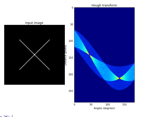
从右边那张图可以看出,有两个交点,说明原图像中有两条直线。
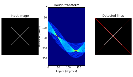
如果我们要把图中的两条直线绘制出来,则需要用到另外一个函数:
skimage.transform.hough_line_peaks(hspace, angles, dists)
用这个函数可以取出峰值点,即交点,也即原图中的直线。
返回的参数与输入的参数一样。我们修改一下上边的程序,在原图中将两直线绘制出来。
import skimage.transform as st
import numpy as np
import matplotlib.pyplot as plt

# 构建测试图片
image = np.zeros((100, 100))  #背景图
idx = np.arange(25, 75)    #25-74序列
image[idx[::-1], idx] = 255  # 线条\
image[idx, idx] = 255        # 线条/

# hough线变换
h, theta, d = st.hough_line(image)

#生成一个一行三列的窗口(可显示三张图片).
fig, (ax0, ax1,ax2) = plt.subplots(1, 3, figsize=(8, 6))
plt.tight_layout()

#显示原始图片
ax0.imshow(image, plt.cm.gray)
ax0.set_title('Input image')
ax0.set_axis_off()

#显示hough变换所得数据
ax1.imshow(np.log(1 + h))
ax1.set_title('Hough transform')
ax1.set_xlabel('Angles (degrees)')
ax1.set_ylabel('Distance (pixels)')
ax1.axis('image')

#显示检测出的线条
ax2.imshow(image, plt.cm.gray)
row1, col1 = image.shape
for _, angle, dist in zip(*st.hough_line_peaks(h, theta, d)):
    y0 = (dist - 0 * np.cos(angle)) / np.sin(angle)
    y1 = (dist - col1 * np.cos(angle)) / np.sin(angle)
    ax2.plot((0, col1), (y0, y1), '-r')
ax2.axis((0, col1, row1, 0))
ax2.set_title('Detected lines')
ax2.set_axis_off()
注意,绘制线条的时候,要从极坐标转换为笛卡尔坐标,公式为:
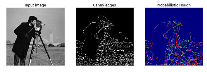
skimage还提供了另外一个检测直线的霍夫变换函数,概率霍夫线变换:
skimage.transform.probabilistic_hough_line(img, threshold=10, line_length=5,line_gap=3)
参数:
img: 待检测的图像。
threshold: 阈值,可先项,默认为10
line_length: 检测的最短线条长度,默认为50
line_gap: 线条间的最大间隙。增大这个值可以合并破碎的线条。默认为10
返回:
lines: 线条列表, 格式如((x0, y0), (x1, y0)),标明开始点和结束点。
下面,我们用canny算子提取边缘,然后检测哪些边缘是直线?
import skimage.transform as st
import matplotlib.pyplot as plt
from skimage import data,feature

#使用Probabilistic Hough Transform.
image = data.camera()
edges = feature.canny(image, sigma=2, low_threshold=1, high_threshold=25)
lines = st.probabilistic_hough_line(edges, threshold=10, line_length=5,line_gap=3)

# 创建显示窗口.
fig, (ax0, ax1, ax2) = plt.subplots(1, 3, figsize=(16, 6))
plt.tight_layout()

#显示原图像
ax0.imshow(image, plt.cm.gray)
ax0.set_title('Input image')
ax0.set_axis_off()

#显示canny边缘
ax1.imshow(edges, plt.cm.gray)
ax1.set_title('Canny edges')
ax1.set_axis_off()

#用plot绘制出所有的直线
ax2.imshow(edges * 0)
for line in lines:
    p0, p1 = line
    ax2.plot((p0[0], p1[0]), (p0[1], p1[1]))
row2, col2 = image.shape
ax2.axis((0, col2, row2, 0))
ax2.set_title('Probabilistic Hough')
ax2.set_axis_off()
plt.show()
python数字图像处理(16):霍夫圆和椭圆变换
在极坐标中,圆的表示方式为:
x=x0+rcosθ
y=y0+rsinθ
圆心为(x0,y0),r为半径,θ为旋转度数,值范围为0-359
如果给定圆心点和半径,则其它点是否在圆上,我们就能检测出来了。在图像中,我们将每个非0像素点作为圆心点,以一定的半径进行检测,如果有一个点在圆上,我们就对这个圆心累加一次。如果检测到一个圆,那么这个圆心点就累加到最大,成为峰值。因此,在检测结果中,一个峰值点,就对应一个圆心点。
霍夫圆检测的函数:
skimage.transform.hough_circle(image, radius)
radius是一个数组,表示半径的集合,如[3,4,5,6]
返回一个3维的数组(radius index, M, N), 第一维表示半径的索引,后面两维表示图像的尺寸。
例1:绘制两个圆形,用霍夫圆变换将它们检测出来。
import numpy as np
import matplotlib.pyplot as plt
from skimage import draw,transform,feature

img = np.zeros((250, 250,3), dtype=np.uint8)
rr, cc = draw.circle_perimeter(60, 60, 50)  #以半径50画一个圆
rr1, cc1 = draw.circle_perimeter(150, 150, 60) #以半径60画一个圆
img[cc, rr,:] =255
img[cc1, rr1,:] =255

fig, (ax0,ax1) = plt.subplots(1,2, figsize=(8, 5))

ax0.imshow(img)  #显示原图
ax0.set_title('origin image')

hough_radii = np.arange(50, 80, 5)  #半径范围
hough_res =transform.hough_circle(img[:,:,0], hough_radii)  #圆变换

centers = []  #保存所有圆心点坐标
accums = []   #累积值
radii = []    #半径

for radius, h in zip(hough_radii, hough_res):
    #每一个半径值,取出其中两个圆
    num_peaks = 2
    peaks =feature.peak_local_max(h, num_peaks=num_peaks) #取出峰值
    centers.extend(peaks)
    accums.extend(h[peaks[:, 0], peaks[:, 1]])
    radii.extend([radius] * num_peaks)

#画出最接近的圆
image =np.copy(img)
for idx in np.argsort(accums)[::-1][:2]:
    center_x, center_y = centers[idx]
    radius = radii[idx]
    cx, cy =draw.circle_perimeter(center_y, center_x, radius)
    image[cy, cx] =(255,0,0)

ax1.imshow(image)
ax1.set_title('detected image')
结果图如下:原图中的圆用白色绘制,检测出的圆用红色绘制。

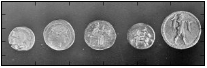
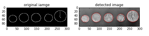
例2,检测出下图中存在的硬币。
import numpy as np
import matplotlib.pyplot as plt
from skimage import data, color,draw,transform,feature,util

image = util.img_as_ubyte(data.coins()[0:95, 70:370]) #裁剪原图片
edges =feature.canny(image, sigma=3, low_threshold=10, high_threshold=50) #检测canny边缘

fig, (ax0,ax1) = plt.subplots(1,2, figsize=(8, 5))

ax0.imshow(edges, cmap=plt.cm.gray)  #显示canny边缘
ax0.set_title('original iamge')

hough_radii = np.arange(15, 30, 2)  #半径范围
hough_res =transform.hough_circle(edges, hough_radii)  #圆变换

centers = []  #保存中心点坐标
accums = []   #累积值
radii = []    #半径

for radius, h in zip(hough_radii, hough_res):
    #每一个半径值,取出其中两个圆
    num_peaks = 2
    peaks =feature.peak_local_max(h, num_peaks=num_peaks) #取出峰值
    centers.extend(peaks)
    accums.extend(h[peaks[:, 0], peaks[:, 1]])
    radii.extend([radius] * num_peaks)

#画出最接近的5个圆
image = color.gray2rgb(image)
for idx in np.argsort(accums)[::-1][:5]:
    center_x, center_y = centers[idx]
    radius = radii[idx]
    cx, cy =draw.circle_perimeter(center_y, center_x, radius)
    image[cy, cx] = (255,0,0)

ax1.imshow(image)
ax1.set_title('detected image')
椭圆变换是类似的,使用函数为:
skimage.transform.hough_ellipse(img,accuracy, threshold, min_size, max_size)
输入参数:
img: 待检测图像。
accuracy: 使用在累加器上的短轴二进制尺寸,是一个double型的值,默认为1
thresh: 累加器阈值,默认为4
min_size: 长轴最小长度,默认为4
max_size: 短轴最大长度,默认为None,表示图片最短边的一半。
返回一个 [(accumulator, y0, x0, a, b, orientation)] 数组,accumulator表示累加器,(y0,x0)表示椭圆中心点,(a,b)分别表示长短轴,orientation表示椭圆方向
例:检测出咖啡图片中的椭圆杯口
import matplotlib.pyplot as plt
from skimage import data,draw,color,transform,feature

#加载图片,转换成灰度图并检测边缘
image_rgb = data.coffee()[0:220, 160:420] #裁剪原图像,不然速度非常慢
image_gray = color.rgb2gray(image_rgb)
edges = feature.canny(image_gray, sigma=2.0, low_threshold=0.55, high_threshold=0.8)

#执行椭圆变换
result =transform.hough_ellipse(edges, accuracy=20, threshold=250,min_size=100, max_size=120)
result.sort(order='accumulator') #根据累加器排序

#估计椭圆参数
best = list(result[-1])  #排完序后取最后一个
yc, xc, a, b = [int(round(x)) for x in best[1:5]]
orientation = best[5]

#在原图上画出椭圆
cy, cx =draw.ellipse_perimeter(yc, xc, a, b, orientation)
image_rgb[cy, cx] = (0, 0, 255) #在原图中用蓝色表示检测出的椭圆

#分别用白色表示canny边缘,用红色表示检测出的椭圆,进行对比
edges = color.gray2rgb(edges)
edges[cy, cx] = (250, 0, 0)

fig2, (ax1, ax2) = plt.subplots(ncols=2, nrows=1, figsize=(8, 4))

ax1.set_title('Original picture')
ax1.imshow(image_rgb)

ax2.set_title('Edge (white) and result (red)')
ax2.imshow(edges)

plt.show()
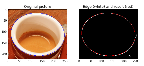
霍夫椭圆变换速度非常慢,应避免图像太大。
python数字图像处理(17):边缘与轮廓
在前面的python数字图像处理(10):图像简单滤波 中,我们已经讲解了很多算子用来检测边缘,其中用得最多的canny算子边缘检测。
本篇我们讲解一些其它方法来检测轮廓。
1、查找轮廓(find_contours)
measure模块中的find_contours()函数,可用来检测二值图像的边缘轮廓。
函数原型为:
skimage.measure.find_contours(array, level)
array: 一个二值数组图像
level: 在图像中查找轮廓的级别值
返回轮廓列表集合,可用for循环取出每一条轮廓。
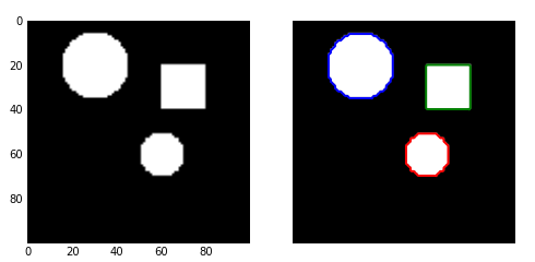
例1:
import numpy as np
import matplotlib.pyplot as plt
from skimage import measure,draw

#生成二值测试图像
img=np.zeros([100,100])
img[20:40,60:80]=1  #矩形
rr,cc=draw.circle(60,60,10)  #小圆
rr1,cc1=draw.circle(20,30,15) #大圆
img[rr,cc]=1
img[rr1,cc1]=1

#检测所有图形的轮廓
contours = measure.find_contours(img, 0.5)

#绘制轮廓
fig, (ax0,ax1) = plt.subplots(1,2,figsize=(8,8))
ax0.imshow(img,plt.cm.gray)
ax1.imshow(img,plt.cm.gray)
for n, contour in enumerate(contours):
    ax1.plot(contour[:, 1], contour[:, 0], linewidth=2)
ax1.axis('image')
ax1.set_xticks([])
ax1.set_yticks([])
plt.show()
结果如下:不同的轮廓用不同的颜色显示
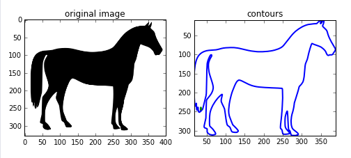
例2:
import matplotlib.pyplot as plt
from skimage import measure,data,color

#生成二值测试图像
img=color.rgb2gray(data.horse())

#检测所有图形的轮廓
contours = measure.find_contours(img, 0.5)

#绘制轮廓
fig, axes = plt.subplots(1,2,figsize=(8,8))
ax0, ax1= axes.ravel()
ax0.imshow(img,plt.cm.gray)
ax0.set_title('original image')

rows,cols=img.shape
ax1.axis([0,rows,cols,0])
for n, contour in enumerate(contours):
    ax1.plot(contour[:, 1], contour[:, 0], linewidth=2)
ax1.axis('image')
ax1.set_title('contours')
plt.show()
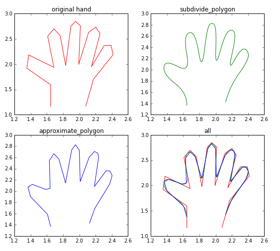
2、逼近多边形曲线
逼近多边形曲线有两个函数:subdivide_polygon()和 approximate_polygon()
subdivide_polygon()采用B样条(B-Splines)来细分多边形的曲线,该曲线通常在凸包线的内部。
函数格式为:
skimage.measure.subdivide_polygon(coords, degree=2, preserve_ends=False)
coords: 坐标点序列。
degree: B样条的度数,默认为2
preserve_ends: 如果曲线为非闭合曲线,是否保存开始和结束点坐标,默认为false
返回细分为的坐标点序列。
approximate_polygon()是基于Douglas-Peucker算法的一种近似曲线模拟。它根据指定的容忍值来近似一条多边形曲线链,该曲线也在凸包线的内部。
函数格式为:
skimage.measure.approximate_polygon(coords, tolerance)
coords: 坐标点序列
tolerance: 容忍值
返回近似的多边形曲线坐标序列。
例:
import numpy as np
import matplotlib.pyplot as plt
from skimage import measure,data,color

#生成二值测试图像
hand = np.array([[1.64516129, 1.16145833],
                 [1.64516129, 1.59375],
                 [1.35080645, 1.921875],
                 [1.375, 2.18229167],
                 [1.68548387, 1.9375],
                 [1.60887097, 2.55208333],
                 [1.68548387, 2.69791667],
                 [1.76209677, 2.56770833],
                 [1.83064516, 1.97395833],
                 [1.89516129, 2.75],
                 [1.9516129, 2.84895833],
                 [2.01209677, 2.76041667],
                 [1.99193548, 1.99479167],
                 [2.11290323, 2.63020833],
                 [2.2016129, 2.734375],
                 [2.25403226, 2.60416667],
                 [2.14919355, 1.953125],
                 [2.30645161, 2.36979167],
                 [2.39112903, 2.36979167],
                 [2.41532258, 2.1875],
                 [2.1733871, 1.703125],
                 [2.07782258, 1.16666667]])

#检测所有图形的轮廓
new_hand = hand.copy()
for _ in range(5):
    new_hand =measure.subdivide_polygon(new_hand, degree=2)

# approximate subdivided polygon with Douglas-Peucker algorithm
appr_hand =measure.approximate_polygon(new_hand, tolerance=0.02)

print("Number of coordinates:", len(hand), len(new_hand), len(appr_hand))

fig, axes= plt.subplots(2,2, figsize=(9, 8))
ax0,ax1,ax2,ax3=axes.ravel()

ax0.plot(hand[:, 0], hand[:, 1],'r')
ax0.set_title('original hand')
ax1.plot(new_hand[:, 0], new_hand[:, 1],'g')
ax1.set_title('subdivide_polygon')
ax2.plot(appr_hand[:, 0], appr_hand[:, 1],'b')
ax2.set_title('approximate_polygon')

ax3.plot(hand[:, 0], hand[:, 1],'r')
ax3.plot(new_hand[:, 0], new_hand[:, 1],'g')
ax3.plot(appr_hand[:, 0], appr_hand[:, 1],'b')
ax3.set_title('all')
python数字图像处理(18):高级形态学处理
形态学处理,除了最基本的膨胀、腐蚀、开/闭运算、黑/白帽处理外,还有一些更高级的运用,如凸包,连通区域标记,删除小块区域等。
1、凸包
凸包是指一个凸多边形,这个凸多边形将图片中所有的白色像素点都包含在内。
函数为:
skimage.morphology.convex_hull_image(image)
输入为二值图像,输出一个逻辑二值图像。在凸包内的点为True, 否则为False
例:
import matplotlib.pyplot as plt
from skimage import data,color,morphology

#生成二值测试图像
img=color.rgb2gray(data.horse())
img=(img<0.5)*1

chull = morphology.convex_hull_image(img)

#绘制轮廓
fig, axes = plt.subplots(1,2,figsize=(8,8))
ax0, ax1= axes.ravel()
ax0.imshow(img,plt.cm.gray)
ax0.set_title('original image')

ax1.imshow(chull,plt.cm.gray)
ax1.set_title('convex_hull image')

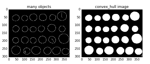
convex_hull_image()是将图片中的所有目标看作一个整体,因此计算出来只有一个最小凸多边形。如果图中有多个目标物体,每一个物体需要计算一个最小凸多边形,则需要使用convex_hull_object()函数。
函数格式:skimage.morphology.convex_hull_object(image, neighbors=8)
输入参数image是一个二值图像,neighbors表示是采用4连通还是8连通,默认为8连通。
例:
import matplotlib.pyplot as plt
from skimage import data,color,morphology,feature

#生成二值测试图像
img=color.rgb2gray(data.coins())
#检测canny边缘,得到二值图片
edgs=feature.canny(img, sigma=3, low_threshold=10, high_threshold=50)

chull = morphology.convex_hull_object(edgs)

#绘制轮廓
fig, axes = plt.subplots(1,2,figsize=(8,8))
ax0, ax1= axes.ravel()
ax0.imshow(edgs,plt.cm.gray)
ax0.set_title('many objects')
ax1.imshow(chull,plt.cm.gray)
ax1.set_title('convex_hull image')
plt.show()
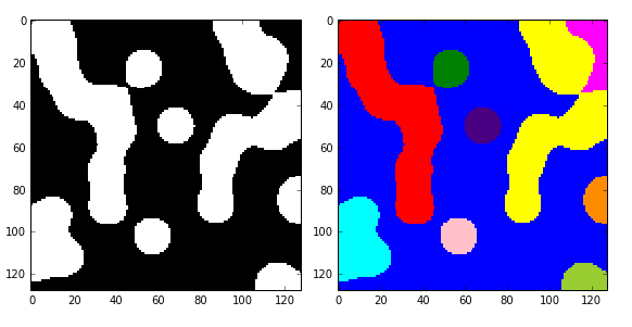
2、连通区域标记
在二值图像中,如果两个像素点相邻且值相同(同为0或同为1),那么就认为这两个像素点在一个相互连通的区域内。而同一个连通区域的所有像素点,都用同一个数值来进行标记,这个过程就叫连通区域标记。在判断两个像素是否相邻时,我们通常采用4连通或8连通判断。在图像中,最小的单位是像素,每个像素周围有8个邻接像素,常见的邻接关系有2种:4邻接与8邻接。4邻接一共4个点,即上下左右,如下左图所示。8邻接的点一共有8个,包括了对角线位置的点,如下右图所示。

在skimage包中,我们采用measure子模块下的label()函数来实现连通区域标记。
函数格式:
skimage.measure.label(image,connectivity=None)
参数中的image表示需要处理的二值图像,connectivity表示连接的模式,1代表4邻接,2代表8邻接。
输出一个标记数组(labels), 从0开始标记。
import numpy as np
import scipy.ndimage as ndi
from skimage import measure,color
import matplotlib.pyplot as plt

#编写一个函数来生成原始二值图像
def microstructure(l=256):
    n = 5
    x, y = np.ogrid[0:l, 0:l]  #生成网络
    mask = np.zeros((l, l))
    generator = np.random.RandomState(1)  #随机数种子
    points = l * generator.rand(2, n**2)
    mask[(points[0]).astype(np.int), (points[1]).astype(np.int)] = 1
    mask = ndi.gaussian_filter(mask, sigma=l/(4.*n)) #高斯滤波
    return mask > mask.mean()

data = microstructure(l=128)*1 #生成测试图片

labels=measure.label(data,connectivity=2)  #8连通区域标记
dst=color.label2rgb(labels)  #根据不同的标记显示不同的颜色
print('regions number:',labels.max()+1)  #显示连通区域块数(从0开始标记)

fig, (ax1, ax2) = plt.subplots(1, 2, figsize=(8, 4))
ax1.imshow(data, plt.cm.gray, interpolation='nearest')
ax1.axis('off')
ax2.imshow(dst,interpolation='nearest')
ax2.axis('off')

fig.tight_layout()
plt.show()
在代码中,有些地方乘以1,则可以将bool数组快速地转换为int数组。
结果如图:有10个连通的区域,标记为0-9
如果想分别对每一个连通区域进行操作,比如计算面积、外接矩形、凸包面积等,则需要调用measure子模块的regionprops()函数。该函数格式为:
skimage.measure.regionprops(label_image)
返回所有连通区块的属性列表,常用的属性列表如下表:
| 属性名称 | 类型 | 描述 |
| area | int | 区域内像素点总数 |
| bbox | tuple | 边界外接框(min_row, min_col, max_row, max_col) |
| centroid | array | 质心坐标 |
| convex_area | int | 凸包内像素点总数 |
| convex_image | ndarray | 和边界外接框同大小的凸包 |
| coords | ndarray | 区域内像素点坐标 |
| Eccentricity | float | 离心率 |
| equivalent_diameter | float | 和区域面积相同的圆的直径 |
| euler_number | int | 区域欧拉数 |
| extent | float | 区域面积和边界外接框面积的比率 |
| filled_area | int | 区域和外接框之间填充的像素点总数 |
| perimeter | float | 区域周长 |
| label | int | 区域标记 |
3、删除小块区域
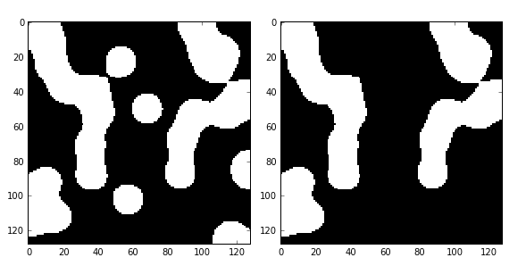
有些时候,我们只需要一些大块区域,那些零散的、小块的区域,我们就需要删除掉,则可以使用morphology子模块的remove_small_objects()函数。
函数格式:skimage.morphology.remove_small_objects(ar, min_size=64, connectivity=1, in_place=False)
参数:
ar: 待操作的bool型数组。
min_size: 最小连通区域尺寸,小于该尺寸的都将被删除。默认为64.
connectivity: 邻接模式,1表示4邻接,2表示8邻接
in_place: bool型值,如果为True,表示直接在输入图像中删除小块区域,否则进行复制后再删除。默认为False.
返回删除了小块区域的二值图像。
import numpy as np
import scipy.ndimage as ndi
from skimage import morphology
import matplotlib.pyplot as plt

#编写一个函数来生成原始二值图像
def microstructure(l=256):
    n = 5
    x, y = np.ogrid[0:l, 0:l]  #生成网络
    mask = np.zeros((l, l))
    generator = np.random.RandomState(1)  #随机数种子
    points = l * generator.rand(2, n**2)
    mask[(points[0]).astype(np.int), (points[1]).astype(np.int)] = 1
    mask = ndi.gaussian_filter(mask, sigma=l/(4.*n)) #高斯滤波
    return mask > mask.mean()

data = microstructure(l=128) #生成测试图片

dst=morphology.remove_small_objects(data,min_size=300,connectivity=1)

fig, (ax1, ax2) = plt.subplots(1, 2, figsize=(8, 4))
ax1.imshow(data, plt.cm.gray, interpolation='nearest')
ax2.imshow(dst,plt.cm.gray,interpolation='nearest')

fig.tight_layout()
plt.show()
在此例中,我们将面积小于300的小块区域删除(由1变为0),结果如下图:
4、综合示例:阈值分割+闭运算+连通区域标记+删除小区块+分色显示
import numpy as np
import matplotlib.pyplot as plt
import matplotlib.patches as mpatches
from skimage import data,filter,segmentation,measure,morphology,color

#加载并裁剪硬币图片
image = data.coins()[50:-50, 50:-50]

thresh =filter.threshold_otsu(image) #阈值分割
bw =morphology.closing(image > thresh, morphology.square(3)) #闭运算

cleared = bw.copy()  #复制
segmentation.clear_border(cleared)  #清除与边界相连的目标物

label_image =measure.label(cleared)  #连通区域标记
borders = np.logical_xor(bw, cleared) #异或
label_image[borders] = -1
image_label_overlay =color.label2rgb(label_image, image=image) #不同标记用不同颜色显示

fig,(ax0,ax1)= plt.subplots(1,2, figsize=(8, 6))
ax0.imshow(cleared,plt.cm.gray)
ax1.imshow(image_label_overlay)

for region in measure.regionprops(label_image): #循环得到每一个连通区域属性集

    #忽略小区域
    if region.area < 100:
        continue

    #绘制外包矩形
    minr, minc, maxr, maxc = region.bbox
    rect = mpatches.Rectangle((minc, minr), maxc - minc, maxr - minr,
                              fill=False, edgecolor='red', linewidth=2)
    ax1.add_patch(rect)
fig.tight_layout()
plt.show()

python数字图像处理(19):骨架提取与分水岭算法
骨架提取与分水岭算法也属于形态学处理范畴,都放在morphology子模块内。
1、骨架提取
骨架提取,也叫二值图像细化。这种算法能将一个连通区域细化成一个像素的宽度,用于特征提取和目标拓扑表示。
morphology子模块提供了两个函数用于骨架提取,分别是Skeletonize()函数和medial_axis()函数。我们先来看Skeletonize()函数。
格式为:skimage.morphology.skeletonize(image)
输入和输出都是一幅二值图像。
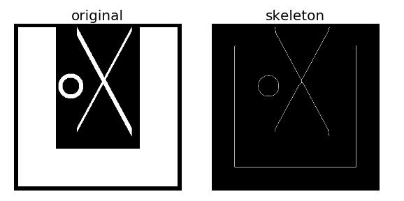
例1:
from skimage import morphology,draw
import numpy as np
import matplotlib.pyplot as plt

#创建一个二值图像用于测试
image = np.zeros((400, 400))

#生成目标对象1(白色U型)
image[10:-10, 10:100] = 1
image[-100:-10, 10:-10] = 1
image[10:-10, -100:-10] = 1

#生成目标对象2(X型)
rs, cs = draw.line(250, 150, 10, 280)
for i in range(10):
    image[rs + i, cs] = 1
rs, cs = draw.line(10, 150, 250, 280)
for i in range(20):
    image[rs + i, cs] = 1

#生成目标对象3(O型)
ir, ic = np.indices(image.shape)
circle1 = (ic - 135)**2 + (ir - 150)**2 < 30**2
circle2 = (ic - 135)**2 + (ir - 150)**2 < 20**2
image[circle1] = 1
image[circle2] = 0

#实施骨架算法
skeleton =morphology.skeletonize(image)

#显示结果
fig, (ax1, ax2) = plt.subplots(nrows=1, ncols=2, figsize=(8, 4))

ax1.imshow(image, cmap=plt.cm.gray)
ax1.axis('off')
ax1.set_title('original', fontsize=20)

ax2.imshow(skeleton, cmap=plt.cm.gray)
ax2.axis('off')
ax2.set_title('skeleton', fontsize=20)

fig.tight_layout()
plt.show()
生成一幅测试图像,上面有三个目标对象,分别进行骨架提取,结果如下:
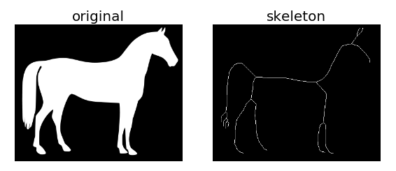
例2:利用系统自带的马图片进行骨架提取
from skimage import morphology,data,color
import matplotlib.pyplot as plt

image=color.rgb2gray(data.horse())
image=1-image #反相
#实施骨架算法
skeleton =morphology.skeletonize(image)

#显示结果
fig, (ax1, ax2) = plt.subplots(nrows=1, ncols=2, figsize=(8, 4))

ax1.imshow(image, cmap=plt.cm.gray)
ax1.axis('off')
ax1.set_title('original', fontsize=20)

ax2.imshow(skeleton, cmap=plt.cm.gray)
ax2.axis('off')
ax2.set_title('skeleton', fontsize=20)

fig.tight_layout()
plt.show()
medial_axis就是中轴的意思,利用中轴变换方法计算前景(1值)目标对象的宽度,格式为:
skimage.morphology.medial_axis(image, mask=None, return_distance=False)
mask: 掩模。默认为None, 如果给定一个掩模,则在掩模内的像素值才执行骨架算法。
return_distance: bool型值,默认为False. 如果为True, 则除了返回骨架,还将距离变换值也同时返回。这里的距离指的是中轴线上的所有点与背景点的距离。
import numpy as np
import scipy.ndimage as ndi
from skimage import morphology
import matplotlib.pyplot as plt

#编写一个函数,生成测试图像
def microstructure(l=256):
    n = 5
    x, y = np.ogrid[0:l, 0:l]
    mask = np.zeros((l, l))
    generator = np.random.RandomState(1)
    points = l * generator.rand(2, n**2)
    mask[(points[0]).astype(np.int), (points[1]).astype(np.int)] = 1
    mask = ndi.gaussian_filter(mask, sigma=l/(4.*n))
    return mask > mask.mean()

data = microstructure(l=64) #生成测试图像

#计算中轴和距离变换值
skel, distance =morphology.medial_axis(data, return_distance=True)

#中轴上的点到背景像素点的距离
dist_on_skel = distance * skel

fig, (ax1, ax2) = plt.subplots(1, 2, figsize=(8, 4))
ax1.imshow(data, cmap=plt.cm.gray, interpolation='nearest')
#用光谱色显示中轴
ax2.imshow(dist_on_skel, cmap=plt.cm.spectral, interpolation='nearest')
ax2.contour(data, [0.5], colors='w')  #显示轮廓线

fig.tight_layout()
plt.show()

2、分水岭算法
分水岭在地理学上就是指一个山脊,水通常会沿着山脊的两边流向不同的“汇水盆”。分水岭算法是一种用于图像分割的经典算法,是基于拓扑理论的数学形态学的分割方法。如果图像中的目标物体是连在一起的,则分割起来会更困难,分水岭算法经常用于处理这类问题,通常会取得比较好的效果。
分水岭算法可以和距离变换结合,寻找“汇水盆地”和“分水岭界限”,从而对图像进行分割。二值图像的距离变换就是每一个像素点到最近非零值像素点的距离,我们可以使用scipy包来计算距离变换。
在下面的例子中,需要将两个重叠的圆分开。我们先计算圆上的这些白色像素点到黑色背景像素点的距离变换,选出距离变换中的最大值作为初始标记点(如果是反色的话,则是取最小值),从这些标记点开始的两个汇水盆越集越大,最后相交于分山岭。从分山岭处断开,我们就得到了两个分离的圆。
例1:基于距离变换的分山岭图像分割
import numpy as np
import matplotlib.pyplot as plt
from scipy import ndimage as ndi
from skimage import morphology,feature

#创建两个带有重叠圆的图像
x, y = np.indices((80, 80))
x1, y1, x2, y2 = 28, 28, 44, 52
r1, r2 = 16, 20
mask_circle1 = (x - x1)**2 + (y - y1)**2 < r1**2
mask_circle2 = (x - x2)**2 + (y - y2)**2 < r2**2
image = np.logical_or(mask_circle1, mask_circle2)

#现在我们用分水岭算法分离两个圆
distance = ndi.distance_transform_edt(image) #距离变换
local_maxi =feature.peak_local_max(distance, indices=False, footprint=np.ones((3, 3)),
                            labels=image)   #寻找峰值
markers = ndi.label(local_maxi)[0] #初始标记点
labels =morphology.watershed(-distance, markers, mask=image) #基于距离变换的分水岭算法

fig, axes = plt.subplots(nrows=2, ncols=2, figsize=(8, 8))
axes = axes.ravel()
ax0, ax1, ax2, ax3 = axes

ax0.imshow(image, cmap=plt.cm.gray, interpolation='nearest')
ax0.set_title("Original")
ax1.imshow(-distance, cmap=plt.cm.jet, interpolation='nearest')
ax1.set_title("Distance")
ax2.imshow(markers, cmap=plt.cm.spectral, interpolation='nearest')
ax2.set_title("Markers")
ax3.imshow(labels, cmap=plt.cm.spectral, interpolation='nearest')
ax3.set_title("Segmented")

for ax in axes:
    ax.axis('off')

fig.tight_layout()
plt.show()

分水岭算法也可以和梯度相结合,来实现图像分割。一般梯度图像在边缘处有较高的像素值,而在其它地方则有较低的像素值,理想情况 下,分山岭恰好在边缘。因此,我们可以根据梯度来寻找分山岭。
例2:基于梯度的分水岭图像分割
import matplotlib.pyplot as plt
from scipy import ndimage as ndi
from skimage import morphology,color,data,filter

image =color.rgb2gray(data.camera())
denoised = filter.rank.median(image, morphology.disk(2)) #过滤噪声

#将梯度值低于10的作为开始标记点
markers = filter.rank.gradient(denoised, morphology.disk(5)) <10
markers = ndi.label(markers)[0]

gradient = filter.rank.gradient(denoised, morphology.disk(2)) #计算梯度
labels =morphology.watershed(gradient, markers, mask=image) #基于梯度的分水岭算法

fig, axes = plt.subplots(nrows=2, ncols=2, figsize=(6, 6))
axes = axes.ravel()
ax0, ax1, ax2, ax3 = axes

ax0.imshow(image, cmap=plt.cm.gray, interpolation='nearest')
ax0.set_title("Original")
ax1.imshow(gradient, cmap=plt.cm.spectral, interpolation='nearest')
ax1.set_title("Gradient")
ax2.imshow(markers, cmap=plt.cm.spectral, interpolation='nearest')
ax2.set_title("Markers")
ax3.imshow(labels, cmap=plt.cm.spectral, interpolation='nearest')
ax3.set_title("Segmented")

for ax in axes:
    ax.axis('off')

fig.tight_layout()
plt.show()


